ARIMA models can also model series with seasonal effects. According to different extraction methods of seasonal effects, it can be further divided into ARIMA additive model and ARIMA multiplicative model.
The ABIMA additive model refers to the additive relationship between the seasonal effect and other effects in the sequence, that is, at
this time, the extraction of various effect information is very easy. Usually, a simple periodic step difference (that is, a step difference with a period as the step size) can fully extract the seasonal information in the sequence, and a simple low-order difference (generally no more than the third order) can fully extract the trend information. The residual sequence after seasonal information and trend information is a stationary sequence, which can be fitted by ARMA model. Therefore, the seasonal additive model is actually to transform the sequence into a stationary sequence through trend difference and seasonal difference, and then fit it. Its model structure is usually as follows:
In the formula,
S is the cycle step size, and d is the difference order used to extract trend information.
is a white noise sequence, and
,
.
, is the qth-order moving average coefficient polynomial.
, is a polynomial of p-order autoregressive coefficients.
The additive model is abbreviated as , or
.
Taking the quarterly unemployment rate of German workers from 1962 to 1991 as an example, the model fitting analysis was carried out with Rstudio software. The data is as follows, and it needs to be saved as a csv file when used.
time x 1962/1/1 1.1 1962/4/1 0.5 1962/7/1 0.4 ###### 0.7 1963/1/1 1.6 1963/4/1 0.6 1963/7/1 0.5 ###### 0.7 1964/1/1 1.3 1964/4/1 0.6 1964/7/1 0.5 ###### 0.7 1965/1/1 1.2 1965/4/1 0.5 1965/7/1 0.4 ###### 0.6 1966/1/1 0.9 1966/4/1 0.5 1966/7/1 0.5 ###### 1.1 1967/1/1 2.9 1967/4/1 2.1 1967/7/1 1.7 ###### 2 1968/1/1 2.7 1968/4/1 1.3 1968/7/1 0.9 ###### 1 1969/1/1 1.6 1969/4/1 0.6 1969/7/1 0.5 ###### 0.7 1970/1/1 1.1 1970/4/1 0.5 1970/7/1 0.5 ###### 0.6 1971/1/1 1.2 1971/4/1 0.7 1971/7/1 0.7 ###### 1 1972/1/1 1.5 1972/4/1 1 1972/7/1 0.9 ###### 1.1 1973/1/1 1.5 1973/4/1 1 1973/7/1 1 ###### 1.6 1974/1/1 2.6 1974/4/1 2.1 1974/7/1 2.3 ###### 3.6 1975/1/1 5 1975/4/1 4.5 1975/7/1 4.5 ###### 4.9 1976/1/1 5.7 1976/4/1 4.3 1976/7/1 4 ###### 4.4 1977/1/1 5.2 1977/4/1 4.3 1977/7/1 4.2 ###### 4.5 1978/1/1 5.2 1978/4/1 4.1 1978/7/1 3.9 ###### 4.1 1979/1/1 4.8 1979/4/1 3.5 1979/7/1 3.4 ###### 3.5 1980/1/1 4.2 1980/4/1 3.4 1980/7/1 3.6 ###### 4.3 1981/1/1 5.5 1981/4/1 4.8 1981/7/1 5.4 ###### 6.5 1982/1/1 8 1982/4/1 7 1982/7/1 7.4 ###### 8.5 1983/1/1 10.1 1983/4/1 8.9 1983/7/1 8.8 ###### 9 1984/1/1 10 1984/4/1 8.7 1984/7/1 8.8 ###### 8.9 1985/1/1 10.4 1985/4/1 8.9 1985/7/1 8.9 ###### 9 1986/1/1 10.2 1986/4/1 8.6 1986/7/1 8.4 ###### 8.4 1987/1/1 9.9 1987/4/1 8.5 1987/7/1 8.6 ###### 8.7 1988/1/1 9.8 1988/4/1 8.6 1988/7/1 8.4 ###### 8.2 1989/1/1 8.8 1989/4/1 7.6 1989/7/1 7.5 ###### 7.6 1990/1/1 8.1 1990/4/1 7.1 1990/7/1 6.9 ###### 6.6 1991/1/1 6.8 1991/4/1 6 1991/7/1 6.2 ###### 6.2
The fitting process is as follows:
1. Draw the time sequence diagram of the observation value sequence
Since observations are recorded in units of quarters, that is, data is recorded 4 times in a year, the frequency is 4 when generating a time series.
m<-read.csv("C:\\Users\\86191\\Desktop\\A1_20.csv",sep=',',header = T)
x<-ts(m$x,start = c(1962,1),frequency = 4)


#绘制时序图
plot(
  x,
  main = "1962年-1991年德国工人季度失业率",
  xlab = "年份",ylab="gov_cons",
  xlim = c(1962,1992),ylim=c(0,11),
  type="o",
  pch=20,
)
Draw the timing diagram as follows: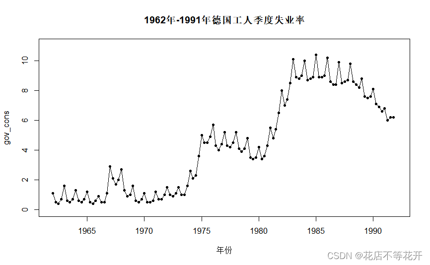
可以看到,该序列既含有长期趋势又含有以年为周期的季节效应。不是平稳序列,接下来需要对其提取趋势,季节效应。
2.差分平稳化
将第1步中的序列记作原序列,则对原序列作1阶差分消除(提取)趋势,再作4步差分消除季节效应的影响。
#绘制一阶差分再以周期时长数目为k的k步差分的时序图
x_diff_4<-diff(diff(x),4)#一阶差分再4步差分
plot(
  x_diff_4,
  main = "1962年-1991年德国工人季度失业率一阶差分再4步差分",
  type="o",
  pch=20,
)
差分后的序列的时序图如下: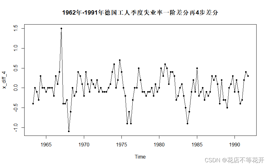
时序图显示,差分后的序列没有明显的趋势或周期,随机波动比较平稳。但这仅是图示法,具有一定的主观性,需要进行ADF检验,白噪声检验判断序列是否具有分析价值。
从时序图可以看到,序列大致在0附近来回波动,所以选择nc类型(无漂移项自回归结构)的ADF检验。
#对一阶差分再以周期时长数目为k的k步差分后的序列进行平稳性检验
library(fBasics)
library(fUnitRoots)
for(i in 0:3) print(
  adfTest(x_diff_4,
          lag=i,
          type="nc",
          title = "1962年-1991年德国工人季度失业率单位根检验"))
结果如下:
Title:
1962年-1991年德国工人季度失业率单位根检验Test Results:
PARAMETER:
Lag Order: 0
STATISTIC:
Dickey-Fuller: -6.7731
P VALUE:
0.01Description:
Sun Nov 13 00:24:28 2022 by user: 86191
Title:
1962年-1991年德国工人季度失业率单位根检验Test Results:
PARAMETER:
Lag Order: 1
STATISTIC:
Dickey-Fuller: -5.5058
P VALUE:
0.01Description:
Sun Nov 13 00:24:28 2022 by user: 86191
Title:
1962年-1991年德国工人季度失业率单位根检验Test Results:
PARAMETER:
Lag Order: 2
STATISTIC:
Dickey-Fuller: -4.8907
P VALUE:
0.01Description:
Sun Nov 13 00:24:28 2022 by user: 86191
Title:
1962年-1991年德国工人季度失业率单位根检验Test Results:
PARAMETER:
Lag Order: 3
STATISTIC:
Dickey-Fuller: -6.2638
P VALUE:
0.01Description:
Sun Nov 13 00:24:28 2022 by user: 86191Warning messages:
1: In adfTest(x_diff_4, lag = i, type = "nc", title = "1962年-1991年德国工人季度失业率单位根检验") :
p-value smaller than printed p-value
2: In adfTest(x_diff_4, lag = i, type = "nc", title = "1962年-1991年德国工人季度失业率单位根检验") :
p-value smaller than printed p-value
3: In adfTest(x_diff_4, lag = i, type = "nc", title = "1962年-1991年德国工人季度失业率单位根检验") :
p-value smaller than printed p-value
4: In adfTest(x_diff_4, lag = i, type = "nc", title = "1962年-1991年德国工人季度失业率单位根检验") :
p-value smaller than printed p-value
结果显示,0-3阶延迟的ADF检验,其p值都显示为0.01,但提示信息告诉我们,真实的p值小于0.01,因此在显著性水平为0.01下,没有充分理由接受ADF检验的原假设:序列非平稳;从而认为差分后的序列是平稳的。接下来进行白噪声检验。
#对一阶差分再以周期时长数目为k的k步差分后的序列进行白噪声检验
for(k in 1:2) print(
  Box.test(x_diff_4,
           lag=6*k,
           type="Ljung-Box"))
结果如下:
Box-Ljung test
data: x_diff_4
X-squared = 43.837, df = 6, p-value = 7.964e-08
Box-Ljung testdata: x_diff_4
X-squared = 51.708, df = 12, p-value = 6.982e-07
检验结果显示,延迟6阶与延迟12阶的白噪声检验的p值都远小于0.001,没有充分理由接受白噪声检验的原假设:序列是白噪声序列;从而认为差分后的序列是非白噪声的。 也就是说,差分后的序列是平稳非白噪声序列,具有分析价值,接下来对差分后的序列进一步拟合ARMA模型。
3、模型拟合
考察差分后序列的自相关图和偏自相关图的性质,给拟合模型定阶。
acf(x_diff_4)#绘制一阶差分再以周期时长数目为k的k步差分自相关图
pacf(x_diff_4)#绘制一阶差分再以周期时长数目为k的k步差分偏相关图
自相关图如下: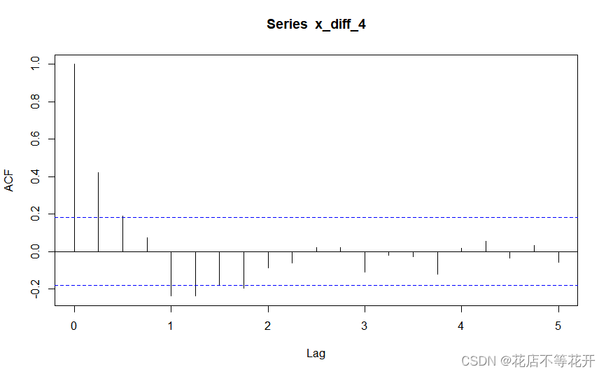 偏自相关图如下:
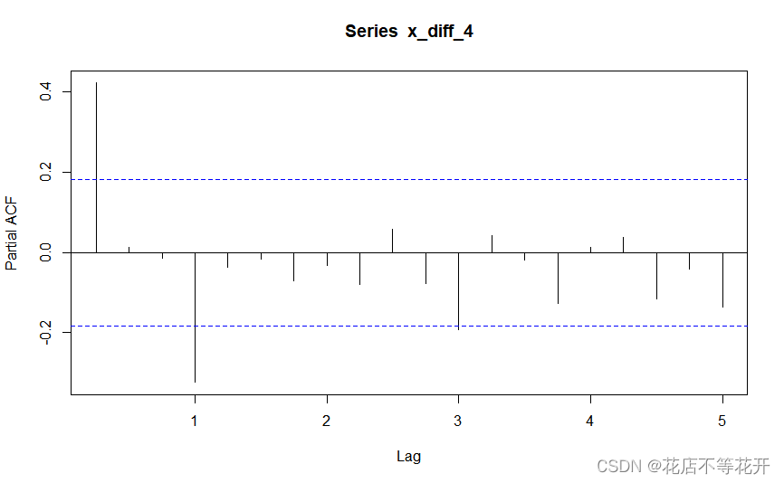
自相关图显示出明显的下滑轨迹,这是典型的拖尾属性。偏自相关图除了1阶和4阶偏自相关系数显著大于2倍标准差,其他阶数的偏自相关系数基本都在2倍标准差范围内波动。所以尝试拟合疏系数模型AR(1,4)。由于第1步中对原序列进行了差分,所以实际上是拟合疏系数的季节加法模型ARIMA((1,4),(1,4),0),或等价表达为ARIMA(1,1,0)(0,1,0)
。使用条件最小二乘法估计模型参数。
#模型拟合-加法季节模型
x_fit<-arima(x,order = c(4,1,0),seasonal=list(order=c(0,1,0),period=4),
             method = "CSS",transform.pars = F,fixed = c(NA,0,0,NA))#实际拟合模型
#include.mean = T:拟合常数项
#include.mean = F:不拟合常数项
#transform.pars:参数估计是否由系统完成
#transform.pars = T:系统根据order设置的模型阶数自动完成参数估计
#transform.pars = F:需要拟合疏系数模型,需要认为干预
#fixed:对疏系数模型指定疏系数的位置
#seasonal:指定季节模型的阶数与季节周期,命令格式为seasonal=list(c(p,d,q),period=周期),d代表以周期为步长的步差分次数
#乘法模型中p,q不全为零,加法模型中p=0,q=0
x_fit
结果如下:
Call:
arima(x = x, order = c(4, 1, 0), seasonal = list(order = c(0, 1, 0), period = 4),
transform.pars = F, fixed = c(NA, 0, 0, NA), method = "CSS")Coefficients:
ar1 ar2 ar3 ar4
0.4507 0 0 -0.2816
s.e. 0.0804 0 0 0.0808sigma^2 estimated as 0.09377: part log likelihood = -27.08
得到该模型的口径如下:
4、模型检验
对差分后的序列的残差进行白噪声检验,以判断拟合的模型是否有效,即序列信息是否提取充分。
#模型的显著性检验(有效性)-残差序列随机性检验
for(k in 1:2) print(
  Box.test(x_fit$residuals,
           lag=6*k,
           type="Ljung-Box"))
结果如下:
Box-Ljung test
data: x_fit$residuals
X-squared = 1.7605, df = 6, p-value = 0.9404
Box-Ljung testdata: x_fit$residuals
X-squared = 9.1286, df = 12, p-value = 0.6919
检验结果显示,延迟6阶与延迟12阶的白噪声检验的p值都远大于0.05的显著性水平,从而认为残差序列为白噪声序列,信息提取充分。接下来对模型的参数进行显著性检验。
#参数显著性检验,即检验参数是否显著非零,拒绝原假设则显著非零
qt(0.975,118)#检验统计量临界值
#ar1系数检验
t1<-0.4507/0.0804
t1
pt(t1,df=118,lower.tail = F)

#ar4检验
t2<-0.2816/0.0808
t2
pt(t2,df=188,lower.tail = T)
检验结果如下:
> #参数显著性检验,即检验参数是否显著非零,拒绝原假设则显著非零
> qt(0.975,118)#检验统计量临界值
[1] 1.980272
> #ar1系数检验
> t1<-0.4507/0.0804
> t1
[1] 5.605721
> pt(t1,df=118,lower.tail = F)
[1] 6.921003e-08
>
> #ar4检验
> t2<-0.2816/0.0808
> t2
[1] 3.485149
> pt(t2,df=188,lower.tail = T)
[1] 0.999694
结果显示,两参数的检验统计量值的绝对值均大于临界值(n为序列长度,m为待估参数个数),即模型参数都显著非零,而第二个参数的检验p值为0.999694是因为R语言中的定义,而并非其p值真是0.999694,可根据其检验统计量的值与临界值判断。
综述,结果显示该模型拟合良好,对序列相关信息的提取充分。
将序列拟合值和序列观察值联合作图,并基于该模型预测1992-2001年德国工人失业率。
#预测
library(forecast)
x.fore<-forecast(x_fit,h=20,level = c(95))#h为预测期数,level为置信度,预测五年
x.fore
plot(x.fore)

#详细预测图-星号是观察值序列,蓝色是两倍95%置信线,实线是拟合值序列
L1<-x.fore$fitted-1.96*sqrt(x_fit$sigma2)
U1<-x.fore$fitted+1.96*sqrt(x_fit$sigma2)
L2<-ts(x.fore$lower[,1],start=1992)#start=预测期数起始年限
U2<-ts(x.fore$upper[,1],start=1992)#start=预测期数起始年限
c1<-min(x,L1,L2)
c2<-max(x,L2,U2)
plot(x,
     type="p",
     pch=8,
     xlim=c(1962,1995),ylim=c(c1,c2))#xlim=c(数据序列起始时间,预测期数终止时间)
lines(x.fore$fitted,col=2,lwd=2)#此时拟合值与观测值同图
lines(x.fore$mean,col=2,lwd=2)
lines(L1,col=4,lty=2)
lines(U1,col=4,lty=2)
lines(L1,col=4,lty=2)
lines(L2,col=4,lty=2)
lines(U2,col=4,lty=2)
1992-2001年德国工人的失业率预测结果如下:
Point Forecast Lo 95 Hi 95
1992 Q1 6.619702 6.01950988 7.219894
1992 Q2 5.862413 4.80487129 6.919955
1992 Q3 5.969028 4.51858464 7.419471
1992 Q4 5.842457 4.05323318 7.631681
1993 Q1 6.143241 3.80612560 8.480356
1993 Q2 5.320323 2.46925775 8.171388
1993 Q3 5.423652 2.12609740 8.721208
1993 Q4 5.331242 1.64292433 9.019560
1994 Q1 5.680910 1.42577545 9.936045
1994 Q2 4.898508 0.06288166 9.734133
1994 Q3 5.021024 -0.36391902 10.405967
1994 Q4 4.927643 -0.96927958 10.824565
1995 Q1 5.263108 -1.30239979 11.828616
1995 Q2 4.462895 -2.77857660 11.704366
1995 Q3 4.571980 -3.30930009 12.453260
1995 Q4 4.472818 -4.00579982 12.951436
1996 Q1 4.809677 -4.40046864 14.019823
1996 Q2 4.015107 -5.93377754 13.963992
1996 Q3 4.130519 -6.52681951 14.787857
1996 Q4 4.035836 -7.29318279 15.364855
The prediction diagram is as follows: 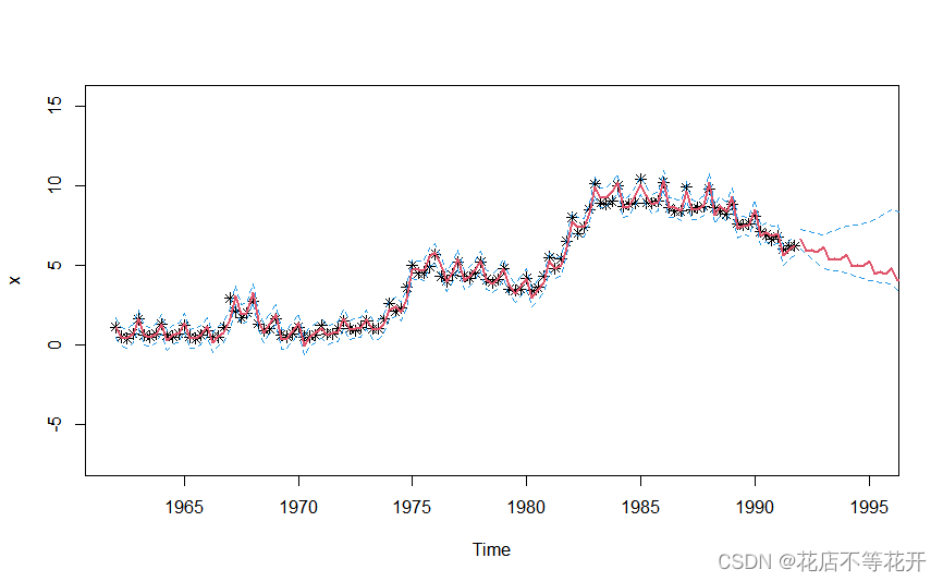 It can also be seen intuitively from the diagram that the model fits the sequence well.