Debezium Daily Sharing Series: Using Data Flows in Databases for Online Machine Learning
1. Background introduction
- Use Debezium to create multiple data streams from the database and use one stream to continuously learn and improve our model, and the second stream to make predictions on the data.
- When a model continuously improves or adjusts to fit the latest data samples, this approach is called online machine learning. Online learning is only suitable for certain use cases, and implementing online variations of a given algorithm can be challenging or even impossible. However, where online learning is possible, it becomes a very powerful tool because it allows one to react to changes in data in real time and avoid the need to retrain and redeploy new models, thus saving time.
- Hardware and operating costs. As data streams become more prevalent, for example with the advent of the Internet of Things, it can be expected that online learning will become increasingly popular. It is generally well suited for analyzing streaming data in possible use cases.
- The goal is not to build the best model for a given use case, but to look at how to build a complete pipeline from inserting data into the database to passing the data to the model and using it for model training and prediction. For simplicity, another well-known data sample often used in machine learning tutorials will be used. You will explore how to classify various iris flowers using an online variant of the k-means clustering algorithm. Use Apache Flink and Apache Spark to process data streams. Both frameworks are very popular data processing frameworks and contain a machine learning library that, among other things, implements the online k-means algorithm. Therefore, we can focus on building a complete pipeline that passes data from the database into a given model, processing it in real time, rather than having to deal with the implementation details of the algorithm.
2. Data set preparation
- You will use the iris flower dataset, and the goal is to determine the species of iris flower based on several measurements of the iris flower: sepal length, sepal width, petal length, and petal width.
- The dataset can be downloaded from various sources. One can take advantage of the fact that it is already preprocessed in e.g. scikit-learn toolkit and use it from there. Each sample row contains a data point (sepal length, sepal width, petal length, and petal width) and label. The label is the number 0, 1, or 2, where 0 represents Iris setosa, 1 represents Iris versicolor, and 2 represents Iris virginica. The data set is small - only 150 data points.
- When loading data into the database, the SQL file is first prepared and later passed to the database. The original data sample needs to be divided into three subsamples - two for training and one for testing. The initial training will use the first training data sample. This data sample is intentionally small so as not to produce good predictions the first time the model is tested, so that you can see how the model's predictions will increase in real time as more data is fed to the model.
- All three SQL files can be generated using the following Python script from the accompanying demo repository.
$ ./iris2sql.py
- train1.sql is automatically loaded into the Postgres database at startup. test.sql and train2.sql will be manually loaded into the database later.
3. Use Apache Flink for classification
First, let's take a look at how to perform online iris classification and learning in Apache Flink. The figure below depicts the high-level architecture of the entire pipeline.
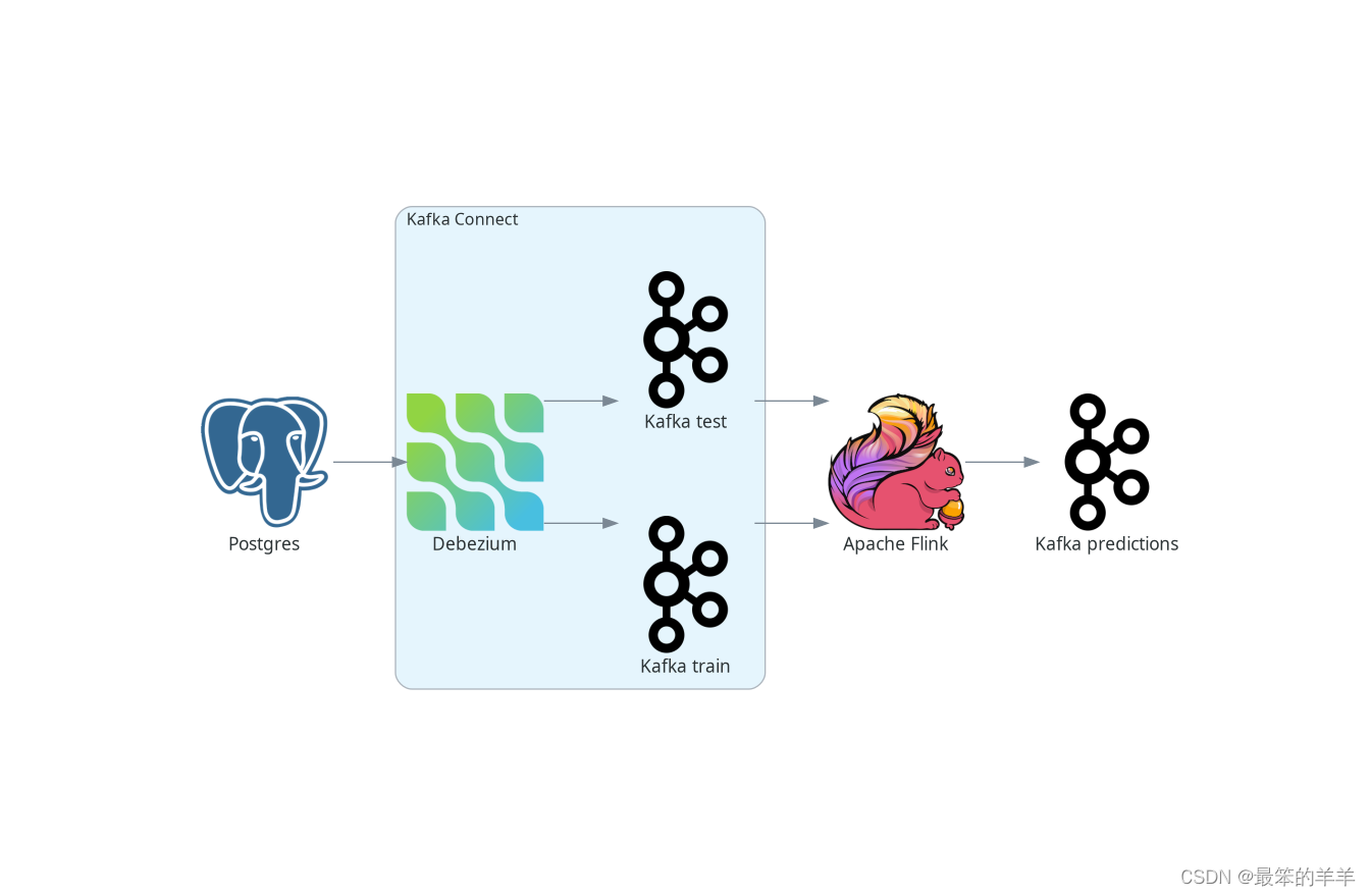
We will use Postgres as our source database. Debezium is deployed as a Kafka Connect source connector, tracking changes in the database and creating a data stream from newly inserted data to Kafka. Kafka sends these streams to Apache Flink, which uses the streaming k-means algorithm for model fitting and data classification. The predictions for the test data stream model are generated as another stream and sent back to Kafka.
Our database contains two tables. The first one stores our training data and the second one stores the test data. Therefore, there are two data streams, one for each table - one for learning and one for the data points to be classified. In real applications, only one table can be used, or conversely, more tables can be used. Even more Debezium connectors can be deployed to merge data from multiple databases.
4. Use Debezium and Kafka as source data streams
Apache Flink has excellent integration with Kafka. Debezium records can be passed, such as JSON records. For creating Flink tables, it even supports Debezium's record format, but for streams, part of the Debezium message needs to be extracted, which contains the newly stored rows in the table. However, this is very easy because Debezium provides SMT, which extracts new record state SMT, and does exactly that. The complete Debezium configuration looks like this:
{


    "name": "iris-connector-flink",
    "config": {


        "connector.class": "io.debezium.connector.postgresql.PostgresConnector",
        "tasks.max": "1",
        "database.hostname": "postgres",
        "database.port": "5432",
        "database.user": "postgres",
        "database.password": "postgres",
        "database.dbname" : "postgres",
        "topic.prefix": "flink",
        "table.include.list": "public.iris_.*",
        "key.converter": "org.apache.kafka.connect.json.JsonConverter",
        "value.converter": "org.apache.kafka.connect.json.JsonConverter",
        "transforms": "unwrap",
        "transforms.unwrap.type": "io.debezium.transforms.ExtractNewRecordState"
    }
}
This configuration captures all tables in the common schema that contain tables starting with the iris_ prefix. Since the training and testing data are stored in two tables, two Kafka topics named flink.public.iris_train and flink.public.iris_test are created respectively. Flink's DataStreamSource represents the incoming data stream. When a record is encoded as JSON, it will be a stream of JSON ObjectNode objects. Building the source stream is very simple:
KafkaSource<ObjectNode> train = KafkaSource.<ObjectNode>builder()
    .setBootstrapServers("kafka:9092")
    .setTopics("flink.public.iris_train")
    .setClientIdPrefix("train")
    .setGroupId("dbz")
    .setStartingOffsets(OffsetsInitializer.earliest())
    .setDeserializer(KafkaRecordDeserializationSchema.of(new JSONKeyValueDeserializationSchema(false)))
    .build();
DataStreamSource<ObjectNode> trainStream = env.fromSource(train, WatermarkStrategy.noWatermarks(), "Debezium train");
Flink mainly runs on the Table abstract object. Furthermore, machine learning models only accept tables as input and predictions are also generated in tabular form. Therefore, the input stream must first be converted into a Table object. First convert the input data stream into a table row stream. You need to define a mapping function that will return a Row object containing a vector of data points. Since the k-means algorithm is an unsupervised learning algorithm, that is, the model does not require the "correct answer" corresponding to the data point, so the label field can be skipped from the vector:
private static class RecordMapper implements MapFunction<ObjectNode, Row> {


    @Override
    public Row map(ObjectNode node) {


        JsonNode payload = node.get("value").get("payload");
        StringBuffer sb = new StringBuffer();
        return Row.of(Vectors.dense(
                        payload.get("sepal_length").asDouble(),
                        payload.get("sepal_width").asDouble(),
                        payload.get("petal_length").asDouble(),
                        payload.get("petal_width").asDouble()));
    }
}
Various parts of Flink's internal pipeline can run on different worker nodes, so type information about the table also needs to be provided. This will create the table object:
StreamTableEnvironment tEnv = StreamTableEnvironment.create(env);
TypeInformation<?>[] types = {

    DenseVectorTypeInfo.INSTANCE};
String names[] = {

    "features"};
RowTypeInfo typeInfo = new RowTypeInfo(types, names);

DataStream<Row> inputStream = trainStream.map(new RecordMapper()).returns(typeInfo);
Table trainTable = tEnv.fromDataStream(inputStream).as("features");
5. Build Flink stream k-means
Once you have a Table object, you can pass it to the model. So create one and pass it a training stream for continuous model training:
OnlineKMeans onlineKMeans = new OnlineKMeans()
    .setFeaturesCol("features")
    .setPredictionCol("prediction")
    .setInitialModelData(tEnv.fromDataStream(env.fromElements(1).map(new IrisInitCentroids())))
    .setK(3);
OnlineKMeansModel model = onlineKMeans.fit(trainTable);
To make things simpler, directly set the number of required clusters to 3 instead of mining the data (e.g. using the elbow method) to find the optimal number of clusters. Also set some initial values for the centers of the clusters instead of using random numbers (Flink provides a convenience method - KMeansModelData.generateRandomModelData() if you want to try using random centers).
In order to obtain predictions on test data, the test stream again needs to be converted into a table. The model converts a table containing test data into a table containing predictions. Finally, convert the prediction to a stream and save it, for example in a Kafka topic:
DataStream<Row> testInputStream = testStream.map(new RecordMapper()).returns(typeInfo);
Table testTable = tEnv.fromDataStream(testInputStream).as("features");
Table outputTable = model.transform(testTable)[0];

DataStream<Row> resultStream = tEnv.toChangelogStream(outputTable);
resultStream.map(new ResultMapper()).sinkTo(kafkaSink);
Now, the application is ready to be built and almost ready to be submitted to Flink for execution. Before doing this, you need to create the required Kafka topic. Although topics can be empty, Flink requires that they at least exist. Because a small portion of the data is included in the Postgres training table when the database starts, Debezium creates the corresponding topic when it registers the Debezium Postgres connector in Kafka Connect. Since the test data table does not yet exist, the topic needs to be created manually in Kafka:
$ docker compose -f docker-compose-flink.yaml exec kafka /kafka/bin/kafka-topics.sh --create --bootstrap-server kafka:9092 --replication-factor 1 --partitions 1 --topic flink.public.iris_test
Now, you are ready to submit your application to Flink.
If you are not using the Docker compose provided in the source code of this demo, please include the Flink ML library in the Flink lib folder, as the ML library is not part of the default Flink distribution.
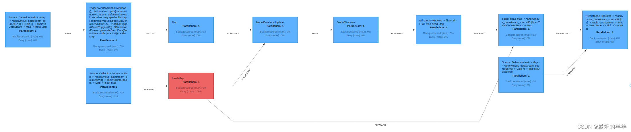
Flink provides a friendly UI, which can be found at http://localhost:8081/. There, among other things, you can check the status of your jobs, such as the job execution plan in an excellent graphical representation:
6. Evaluation model
From the user's perspective, all interactions with the model occur by inserting new records into the database or reading Kafka topics with predictions. Since a very small initial training data sample is already created when the database is started, model predictions can be checked directly by inserting a test data sample into the database:
$ psql -h localhost -U postgres -f postgres/iris_test.sql
The insert generates an instant stream of test data in Kafka, passes it into the model and sends the predictions back to the iris_predictions Kafka topic. When training the model on a very small dataset with only two clusters, the predictions are inaccurate. The chart below shows our preliminary forecast:
[5.4, 3.7, 1.5, 0.2] is classified as 0
[4.8, 3.4, 1.6, 0.2] is classified as 0
[7.6, 3.0, 6.6, 2.1] is classified as 2
[6.4, 2.8, 5.6, 2.2] is classified as 2
[6.0, 2.7, 5.1, 1.6] is classified as 2
[5.4, 3.0, 4.5, 1.5] is classified as 2
[6.7, 3.1, 4.7, 1.5] is classified as 2
[5.5, 2.4, 3.8, 1.1] is classified as 2
[6.1, 2.8, 4.7, 1.2] is classified as 2
[4.3, 3.0, 1.1, 0.1] is classified as 0
[5.8, 2.7, 3.9, 1.2] is classified as 2
In our example, the correct answer would be:
[5.4, 3.7, 1.5, 0.2] is 0
[4.8, 3.4, 1.6, 0.2] is 0
[7.6, 3.0, 6.6, 2.1] is 2
[6.4, 2.8, 5.6, 2.2] is 2
[6.0, 2.7, 5.1, 1.6] is 1
[5.4, 3.0, 4.5, 1.5] is 1
[6.7, 3.1, 4.7, 1.5] is 1
[5.5, 2.4, 3.8, 1.1] is 1
[6.1, 2.8, 4.7, 1.2] is 1
[4.3, 3.0, 1.1, 0.1] is 0
[5.8, 2.7, 3.9, 1.2] is 1
When comparing the results, only 5 out of 11 data points were correctly classified due to the size of the initial sample training data. On the other hand, since you don't start with completely random clusters, the predictions aren't completely wrong either.
What happens when the model is fed more training data:
$ psql -h localhost -U postgres -f postgres/iris_train2.sql
To see the updated predictions, insert the same test data sample into the database again:
psql -h localhost -U postgres -f postgres/iris_test.sql
The following predictions are much better since all three categories have been provided. It also correctly classified 7 out of 11 data points.
[5.4, 3.7, 1.5, 0.2] is classified as 0
[4.8, 3.4, 1.6, 0.2] is classified as 0
[7.6, 3.0, 6.6, 2.1] is classified as 2
[6.4, 2.8, 5.6, 2.2] is classified as 2
[6.0, 2.7, 5.1, 1.6] is classified as 2
[5.4, 3.0, 4.5, 1.5] is classified as 2
[6.7, 3.1, 4.7, 1.5] is classified as 2
[5.5, 2.4, 3.8, 1.1] is classified as 1
[6.1, 2.8, 4.7, 1.2] is classified as 2
[4.3, 3.0, 1.1, 0.1] is classified as 0
[5.8, 2.7, 3.9, 1.2] is classified as 1
Since the entire data sample is very small, for further model training, the second training data sample can be reused:
$ psql -h localhost -U postgres -f postgres/iris_train2.sql
$ psql -h localhost -U postgres -f postgres/iris_test.sql
This leads to the following prediction.
[5.4, 3.7, 1.5, 0.2] is classified as 0
[4.8, 3.4, 1.6, 0.2] is classified as 0
[7.6, 3.0, 6.6, 2.1] is classified as 2
[6.4, 2.8, 5.6, 2.2] is classified as 2
[6.0, 2.7, 5.1, 1.6] is classified as 2
[5.4, 3.0, 4.5, 1.5] is classified as 1
[6.7, 3.1, 4.7, 1.5] is classified as 2
[5.5, 2.4, 3.8, 1.1] is classified as 1
[6.1, 2.8, 4.7, 1.2] is classified as 1
[4.3, 3.0, 1.1, 0.1] is classified as 0
[5.8, 2.7, 3.9, 1.2] is classified as 1
It is now found that 9 out of 11 data points are correctly classified. While this is still not a stellar result, it is expected that the result will only be partially accurate since it is only a prediction. The main motivation here is to demonstrate the entire process and prove that the model can improve predictions when new data is added without the need to retrain and redeploy the model.
7. Use Apache Spark for classification
From a user's perspective, Apache Spark is very similar to Flink, and the implementation is also very similar.
Spark has two streaming models: the older DStreams (now legacy) and the newer and recommended Structured Streaming model. However, since the streaming k-means algorithm included in the Spark ML library only works with DStreams, a DStream is used in this example for simplicity. A better approach is to use structured streaming and implement streaming k-means yourself.
Spark supports streaming from Kafka using DStreams. However, writing a DStream back to Kafka is not supported, and although it is possible, it is not trivial.
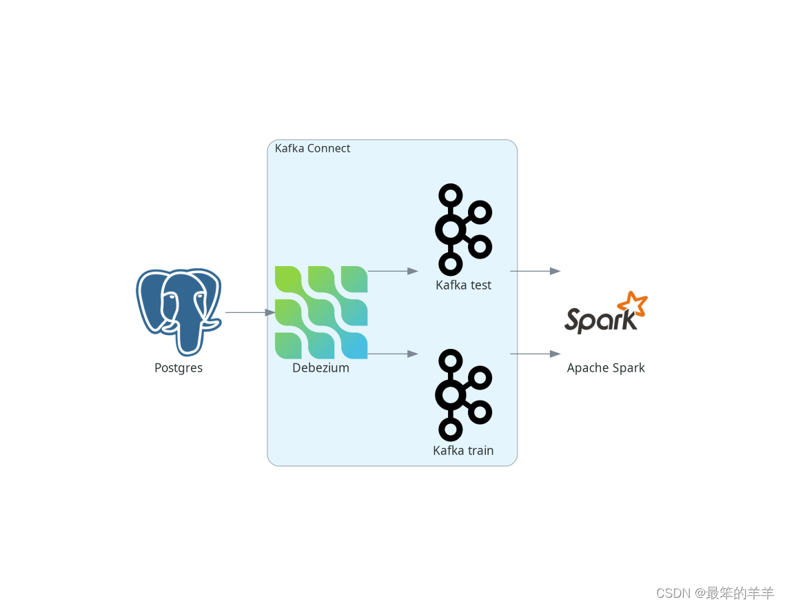
Again, to keep it simple, skip the last part and just write the predictions to the console instead of writing them back to Kafka. The overall picture of the pipeline looks like this:
8. Define data flow
Similar to Flink, creating a Spark stream from a Kafka stream is very simple and most parameters are self-explanatory:
Set<String> trainTopic = new HashSet<>(Arrays.asList("spark.public.iris_train"));
Set<String> testTopic = new HashSet<>(Arrays.asList("spark.public.iris_test"));
Map<String, Object> kafkaParams = new HashMap<>();
kafkaParams.put(ConsumerConfig.BOOTSTRAP_SERVERS_CONFIG, "kafka:9092");
kafkaParams.put(ConsumerConfig.GROUP_ID_CONFIG, "dbz");
kafkaParams.put(ConsumerConfig.AUTO_OFFSET_RESET_CONFIG, "earliest");
kafkaParams.put(ConsumerConfig.KEY_DESERIALIZER_CLASS_CONFIG, StringDeserializer.class);
kafkaParams.put(ConsumerConfig.VALUE_DESERIALIZER_CLASS_CONFIG, StringDeserializer.class);

JavaInputDStream<ConsumerRecord<String, String>> trainStream = KafkaUtils.createDirectStream(
        jssc,
        LocationStrategies.PreferConsistent(),
        ConsumerStrategies.Subscribe(trainTopic, kafkaParams));
JavaDStream<LabeledPoint> train = trainStream.map(ConsumerRecord::value)
        .map(SparkKafkaStreamingKmeans::toLabeledPointString)
        .map(LabeledPoint::parse);
In the last line, the Kafka stream is converted into a marker stream, which is used by the Spark ML library to process its ML model. Markpoint should be a string formatted as a data point label separated by a comma from a space-separated data point value. So the map function looks like this:
private static String toLabeledPointString(String json) throws ParseException {


    JSONParser jsonParser = new JSONParser();
    JSONObject o = (JSONObject)jsonParser.parse(json);
    return String.format("%s, %s %s %s %s",
            o.get("iris_class"),
            o.get("sepal_length"),
            o.get("sepal_width"),
            o.get("petal_length"),
            o.get("petal_width"));
}
It still holds true that k-means is an unsupervised algorithm and does not use data point labels. However, it is convenient to pass them to the LabeledPoint class so that we can display them later along with the model predictions.
We then chain a mapping function to parse the string and create a labeled data point from it. In this case, it is a built-in function of Spark LabeledPoint.
Contrary to Flink, Spark does not require Kafka topics to pre-exist, so when deploying a model, the topic does not have to be created. Once the tables containing your test data are created and populated, you can let Debezium create them.
9. Define and evaluate models
Defining a streaming k-means model is very similar to Flink:
StreamingKMeans model = new StreamingKMeans()
        .setK(3)
        .setInitialCenters(initCenters, weights);
model.trainOn(train.map(lp -> lp.getFeatures()));
Also, in this case, directly set the number of clusters to 3 and provide the clusters with the same initial center point. Also only pass data points for training, not labels.
As mentioned above, we can use labels to display them along with predictions:
JavaPairDStream<Double, Vector> predict = test.mapToPair(lp -> new Tuple2<>(lp.label(), lp.features()));
model.predictOnValues(predict).print(11);
Prints 11 stream elements to the console on the resulting stream with predictions since this is the size of the test sample. As with Flink, results may be better after initial training on very small data samples. The first number in the tuple is the data point label, while the second number is the corresponding prediction made by the model:
spark_1      | (0.0,0)
spark_1      | (0.0,0)
spark_1      | (2.0,2)
spark_1      | (2.0,2)
spark_1      | (1.0,0)
spark_1      | (1.0,0)
spark_1      | (1.0,2)
spark_1      | (1.0,0)
spark_1      | (1.0,0)
spark_1      | (0.0,0)
spark_1      | (1.0,0)
However, when more training data is provided, the predictions get better:
spark_1      | (0.0,0)
spark_1      | (0.0,0)
spark_1      | (2.0,2)
spark_1      | (2.0,2)
spark_1      | (1.0,1)
spark_1      | (1.0,1)
spark_1      | (1.0,2)
spark_1      | (1.0,0)
spark_1      | (1.0,1)
spark_1      | (0.0,0)
spark_1      | (1.0,0)
If you again pass a second training data sample for training, the model makes correct predictions for the entire test sample:
---
spark_1      | (0.0,0)
spark_1      | (0.0,0)
spark_1      | (2.0,2)
spark_1      | (2.0,2)
spark_1      | (1.0,1)
spark_1      | (1.0,1)
spark_1      | (1.0,1)
spark_1      | (1.0,1)
spark_1      | (1.0,1)
spark_1      | (0.0,0)
spark_1      | (1.0,1)
----
The prediction is the number of clusters created by the k-means algorithm, regardless of the labels in the data sample. This means that for example (0.0,1) is not necessarily a wrong prediction. A data point with label 0 might be assigned to the correct cluster, but Spark internally labels it as cluster number 1. This needs to be kept in mind when evaluating models.
Therefore, similar to Flink, when passed more training data, you will get better results without the need to retrain and redeploy the model. In this case, better results than the Flink model were obtained.
10. Conclusion
- Shows how to pass data from the database to Apache Flink and Apache Spark in real time as a data stream. In both cases, the integration is easy to set up and works well.
- This is demonstrated in the example that allows us to use an online learning algorithm, namely the online k-means algorithm, to highlight the power of data streams. Online machine learning allows us to make real-time predictions on data streams and improve or adjust models as soon as new training data arrives. Model tuning does not require retraining any model on a separate computing cluster and redeploying new models, making ML-ops simpler and more cost-effective.