[Reinforcement Learning] Detailed explanation of value function algorithm DQNs [Vanilla DQN & Double DQN & Dueling DQN]

DQNs【Vanilla DQN & Double DQN & Dueling DQN】

​ In the Q-learning algorithm explained in Reinforcement Learning with Code [Code 1. Tabular Q-learning] , we established a matrix to store all actions $Table\; of\; Q$ values. Each action in the table has value $Q(s,a)$ means in state $Select\; an\; action\; under\; s$ and continue to follow a strategy to predict the expected return. However, this method of using tables to store action values ​​is only applicable when the state and actions of the environment are discrete and the space is relatively small. This approach is not applicable when the number of states or actions is very large. For example, when the state is an RGB image, assume the image size is $210\times 160\times 3$ , there are a total of $256^{(210\times 160\times 3)}$ states, it is unrealistic to store a value table of this order of magnitude in a computer. What's more, when states or actions are continuous, there are infinite state-action pairs, and we cannot use this table form to record the $Q$ value.

​ For this situation, we need to use function fitting method to estimate the value $Q$ , this complex$The\; Q$ value table is treated as data, using a parameterized function$Q_{}$to fit these data. Obviously, this method of function fitting has a certain loss of accuracy, so it is called an approximation method. The DQN algorithm we are going to introduce today can be used to solve discrete action problems in continuous states.

1. Introduction to DQN and its variants

1.1 Vanilla DQN

Vanilla DQN is the most basic DQN algorithm. The objective function that needs to be optimized in Q-learning is
$$\underset{i}{\min }J(\theta )=E\left[\right(R+c\underset{a}{\max }Q(S^{\prime },a;i)-Q(S,A;\theta )\left)\right]$$
在Q-learning中的TD target是 $Y_t^Q=R_{t+1}+c{\max }_{a}Q(S_{t+1},a;i_t)$ , if you directly update the above network, you need to consider very complicated issues. Two networks are used in DQN to simplify this process.

Vallina DQN uses two tricks:

• Experience Replay maintains an experience pool that combines the experience of the agent's interaction with the environment $(s,a,r,s^{\prime },\text{done})$ is stored in the experience pool, and then the experience is taken out from the maintained experience pool for training. This has two benefits. First, because the problem we solve is modeled as a Markov Decision Process (MDP). The data obtained by interactive sampling in MDP itself does not satisfy the independence assumption, because the state at this moment is related to the state at the previous moment. Non-independent and identically distributed data has a great impact on training neural networks, making the neural network fit to the most recently trained data. Using experience replay can break the correlation between samples and make them satisfy the independence assumption. Second, improve sample efficiency. Each sample can be used multiple times, which is very suitable for gradient learning of deep neural networks.

• Two Networks , Vanilla DQN, in order to solve the update timing problem in training, before introducing two sets of networks, it is hoped that the parameters of the network $\theta$能够跟踪$Y_t^Q=R_{t+1}+c{\max }_{a}Q(S_{t+1},a;i_t)$，其中$Y_t^Q$It is called TD target. After introducing two sets of networks, they are divided into training network and target network, and the network parameters are respectively represented by $\theta$和$i^{-}$ to express, the ultimate goal of Vanilla DQN is to make the target network$i^{The\; output\; of\; -}$ can approximate
  $$Y_t^D=R_{t+1}+c\underset{a}{\max }Q(S_{t+1},a;i^{-})$$
  So after this, the objective function to be optimized becomes
  $$\underset{i}{\min }J(\theta )=E\left[\right(R+c\underset{a}{\max }Q(S^{\prime },a;i^{-})-Q(S,A;\theta )\left)\right]$$
  We use this objective function as the loss function that Vallina DQN needs to optimize to update the training network parameters$\theta$ , then every$\tau$ generation, the training network parameters$\theta$ is copied to the target network$i^{-}$。

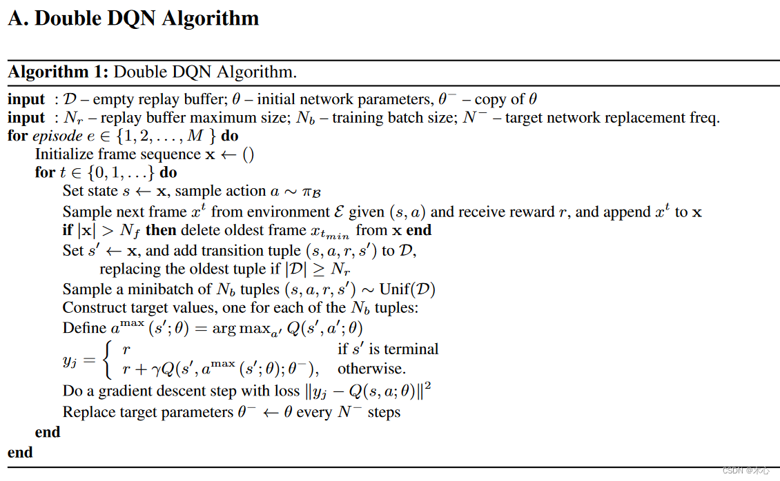
1.2 Double DQN

Double DQN was proposed to solve the problem of overestimation of Q value (overestimation) of Vallina DQN in practical applications. The optimized TD target of Vallina DQN is
$$Y_t^D=R_{t+1}+c\underset{a}{\max }Q(S_{t+1},a;i^{-})$$
其中${\max }_{a}Q(S_{t+1},a;i^{-})$is determined by the parameters of the target network$i^{-Calculated}$ , then we can get the optimal action$a^{\ast }=\arg {\max }_{a}Q(S_{t+1},a;i^{-})$, bringing back the optimal action, then we can rewrite the above formula as
$$Y_t^D=R_{t+1}+\gamma Q(S_{t+1},\arg \underset{a}{\max }Q(S_{t+1},a;i^{-});i^{-})$$
In other words$The\; max$ operation can actually be divided into two parts. First, select the state$S_{t+1}$The optimal action $a^{\ast }=\arg {\max }_{a}Q(S_{t+1},a;i^{-})$Then calculate the value of the action$Q(S_{t+1},a^{\ast };i^{-})$. But when both parts are trained using the same set of Q networks, each calculation results in the maximum value of all action values ​​currently estimated in the neural network. Considering that the Q value estimated by the neural network itself will produce positive or negative errors at certain times, the neural network will accumulate positive errors in the DQN update method.

In order to solve this problem, Double DQN proposes to use two independent networks to estimate ${\max }_a{Q}^{\ast }(S_{t+1},A_{t+1})$ . The specific method is to convert the original${\max }_{a}Q(S_{t+1},a;i^{-})$更改为$Q(S_{t+1},\arg {\max }_{a}Q(S_{t+1},a;i),i^{-})$. That is, using a set of training network$\theta$ to select the action with the greatest value, using the target neural network$i^{-}$ to calculate the value of the action. In this way, even if a certain action of one set of neural networks has a serious overestimation problem, due to the existence of another set of neural networks, this action will ultimately prevent the Q value from being overestimated. Then we can write the TD target of Double DQN as
$$Y_t^{DD}=R_{t+1}+\gamma Q(S_{t+1},\arg \underset{a}{\max }Q(S_{t+1},a;i);i^{-})$$
Pesudocode

1.3 Dueling DQN

Dueling DQN is a variant algorithm of Vanilla DQN. It only makes minor changes on the basis of traditional Vanilla DQN, but greatly improves the performance capabilities of DQN. Specifically, Dueling DQN does not directly estimate the Q-value function, but indirectly obtains the Q-value function by estimating the V state value function and the A advantage function . Dueling DQN very innovatively introduces the concept of advantage function. Before introducing the advantage function, we first review the definitions of action value function Q and state value function V: Q π ( s , a ) = E [ R
$$\begin{gathered} Q^{\pi }(s,a)=E[R_t|s_t=s,a_t=a,p\left] \\ {V}^{\pi }\right(s,a)={\mathbb{E}}_{a\sim \pi }[Q^{\pi }(s,a)] \end{gathered}$$
Advantage function (Advantage function) is defined as
$$A^{\pi }(s,a)=Q^{\pi }(s,a)-V^{\pi }\left(s\right)$$
We take the dominance function as$a\sim \pi$的expectation，则有
$$A^{\pi }(s,a)={\mathbb{E}}_{a\sim \pi }[Q^{\pi }(s,a)]-E_{a\sim \pi }\left[Q^{\pi }\right(s,a)]=0Intuitively$$
, the state value function V measures the state$How\; good\; or\; bad\; s$ is, however, the Q function measures the state$To\; select\; the\; value\; of\; a\; specific\; operation\; under\; s$ , the advantage function A subtracts the state value V from the Q function to obtain the relative degree of importance of each action. For the deterministic policy$\pi$ , the optimal action can be expressed as
$$a^{\ast }=\arg \underset{a^{\prime }\in \mathcal{A}}{\max }Q(s,a^{\prime })$$
and because the strategy is deterministic, then
$$Q(s,a^{\ast })=V\left(s\right)$$
then for the optimal action$a^{The\; advantage\; function\; of\; \ast }$ is
$$A(s,a^{\ast })=0$$
Next, we will introduce the innovation in network structure. In Dueling DQN, in order to realize the above potential function, the network structure has also changed.

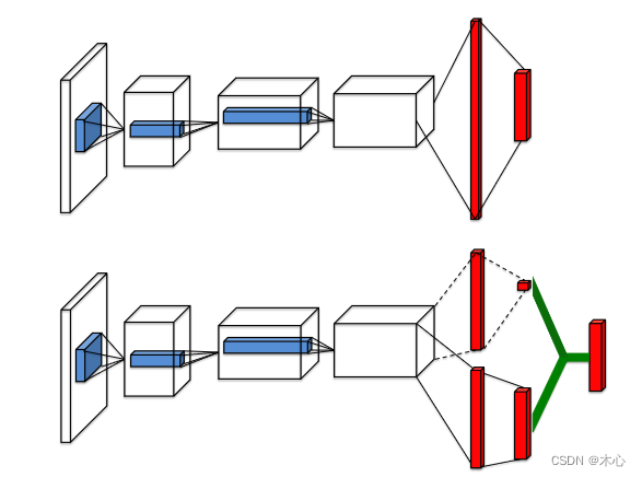
In the figure, the network structure at the top is the structure of DQN, and the network structure at the bottom is the structure of Dueling DQN. The Dueling network has two streams to estimate the state value V (scalar) and the advantage A (vector) of each action respectively; the green output module implements the equation $A^{\pi }(s,a)=Q^{\pi }(s,a)-V^{\pi }\left(s\right)$to combine them. Combined with the above network structure, we add the parameters of the network structure to rewrite the expression of the advantage function A
$$\begin{array}{rl}A(s,a;i,a)& =Q(s,a;i,a,b)-V(s;i,b)\\ Q(s,a;i,a,b& =A(s,a;i,a)+V(s;i,b\end{array}$$
Among them, $\theta$ represents the parameters of the previous shared network structure,$a,\beta$ represents the network structure parameters of the two flows respectively. However, in the above formula, there is a problem of uncertainty about the uniqueness of V value and A value. In order to solve this problem, we add a constant C of any size to the same Q value, and then subtract C from all A values. The Q value obtained in this way remains unchanged, which leads to instability in training. In order to solve this problem, Dueling DQN forces the high-quality function output of the optimal action to be set to 0, that is, Q ( s , a ; θ ,
$$Q(s,a;i,a,b)=V(s;i,b)+(A(s,a;i,a)-\underset{a^{\prime }\in \mathcal{A}}{\max }A(s,a^{\prime };i,\alpha \left)\right)$$
According to the previous analysis, we know that for the optimal action$a^{\ast }$ , the value of the advantage function is 0, that is,$A(s,a^{\ast })=0$ , for the optimal action$a^{\ast }$
$$\begin{array}{rl}{a}^{\ast }& =\arg \underset{a^{\prime }\in \mathcal{A}}{\max }Q(s,a^{\prime };i,a,b)\\ & =\arg \underset{a^{\prime }\in A}{\max }[A(s,a;i,a)+V(s;i,b)]\\ & =\arg \underset{a^{\prime }\in \mathcal{A}}{\max }A(s,a;i,a\end{array}$$
Then the optimal action $a^{\ast }$ Specifically, then
$$Q(s,a^{\ast };i,a,b)=V(s;i,\beta )$$
Therefore, decoupling is successfully achieved, a flow$V(s;i,\beta )$ provides an estimate of the value of the state, another stream$A(s,a;i,\alpha )$ realizes the estimation of advantage value.

In practice, we often replace the maximum (max) operation with the average operation, which is more stable, as follows
$$Q(s,a;i,a,b)=V(s;i,b)+(A(s,a;i,a)-\frac{1}{|\mathcal{A}|}A(s,a^{\prime };i,\alpha \left)\right)$$
Use the above Q value function to calculate the TD target in Vanilla DQN to get the TD target of Dueling DQN. Then update it according to the remaining methods of Vanilla DQN, and we will get the complete algorithm of Dueling DQN.
$$Y_t^{}=R_{t+1}+c\underset{a}{\max }Q(S_{t+1},a;i,a,\beta )$$
and$Q(S_{t+1},a;i,a,Ώد$以range换成average产产ide结果，那么完整的t TARGET就成了
$$Y_t^{}=R_{t+1}+\gamma V(s;i,b)+c\underset{a}{\max }(A(s,a;i,a)-\frac{1}{|\mathcal{A}|}A(s,a^{\prime };i,\alpha \left)\right)$$
with$Q(S_{t+1},a;i,a,\beta )$ can also be replaced by the demerit generated by the max operation, then the complete TD target becomes
$$Y_t^{}=R_{t+1}+\gamma V(s;i,b)+c\underset{a}{\max }(A(s,a;i,a)-\underset{a^{\prime }\in \mathcal{A}}{\max }A(s,a^{\prime };i,a\left)\right)$$

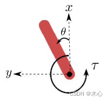
2. Introduction to Gym environment

In order to better observe the problem of Q value estimation overestimation in DQN, we use Pendulum-v1the environment in gym (see the official website for details ). Note that the version of gym here is v26,

The data annotation for the inverted pendulum is as follows

2.1 Observation Space

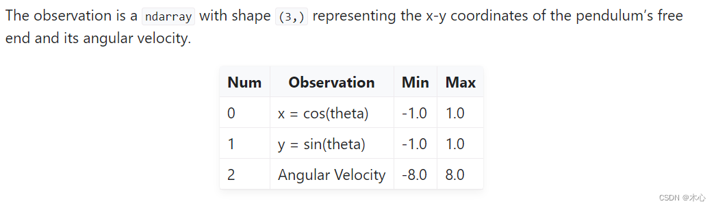
2.2 Reward Function

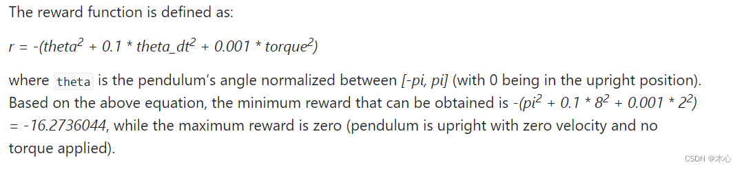
The reward function of this environment is
$$-(i^2+0.1{\dot{i}}^2+0.001a^2)$$
The reward is 0 when the inverted pendulum remains stationary upwards, and the rewards of the inverted pendulum at other positions are negative, so the action value Q will not exceed 0 in this environment.

2.3 Action Space

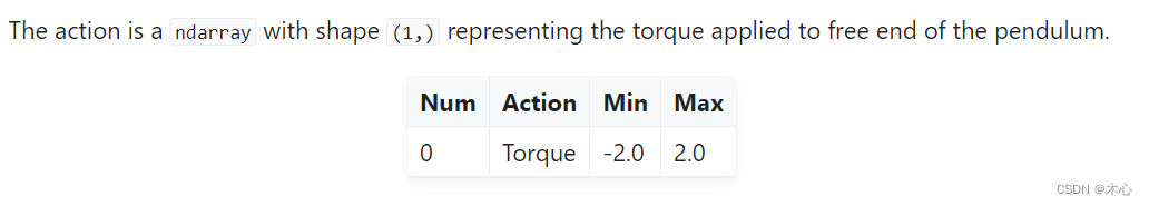
The action space is a continuous value and is the torque acting on the end of the inverted pendulum. However, DQNs can only be used to handle discrete action space environments, so we cannot directly use DQNs to handle the inverted pendulum environment. However, the inverted pendulum environment will make it easier to verify that Vanilla DQN has the problem of overestimating the Q value. In order to enable DQNs to handle this continuous action space environment, we can use the method of discretizing the continuous action space to achieve a pseudo-continuous effect.

import gym
env_name = 'Pendulum-v1'
env = gym.make(id=env_name)
print("The minimum of action space is ", env.action_space.low[0])
print("The maximum of action space is ", env.action_space.high[0])

def dis2con(discrete_action, action_dim, env):
    action_upbound = env.action_space.high[0]
    action_lowbound = env.action_space.low[0]
    return action_lowbound + discrete_action * (action_upbound - action_lowbound) / (action_dim - 1)

# 示例将[-2.0,2.0]的连续动作空间转换成30维度离散动作空间
action_dim = 30 
discrete_action =  list(range(action_dim))
continue_action = []
for da in discrete_action:
    continue_action.append(dis2con(da, action_dim, env))
print(discrete_action)
print(continue_action)
env.close()

The results are as follows

The minimum of action space is  -2.0
The maximum of action space is  2.0
[0, 1, 2, 3, 4, 5, 6, 7, 8, 9, 10, 11, 12, 13, 14, 15, 16, 17, 18, 19, 20, 21, 22, 23, 24, 25, 26, 27, 28, 29]
[-2.0, -1.8620689655172413, -1.7241379310344827, -1.5862068965517242, -1.4482758620689655, -1.3103448275862069, -1.1724137931034484, -1.0344827586206895, -0.896551724137931, -0.7586206896551724, -0.6206896551724137, -0.48275862068965525, -0.3448275862068966, -0.2068965517241379, -0.06896551724137923, 0.06896551724137945, 0.2068965517241379, 0.34482758620689635, 0.48275862068965525, 0.6206896551724137, 0.7586206896551726, 0.896551724137931, 1.0344827586206895, 1.1724137931034484, 1.3103448275862069, 1.4482758620689653, 1.5862068965517242, 1.7241379310344827, 1.8620689655172415, 2.0]

3. DQNs Code

In this section, we formally implement Vanilla DQN, Double DQN and Dueling DQN and observe and compare their effects.

import random
import collections
import torch
import torch.nn.functional as F
import numpy as np
from tqdm import tqdm
import gym
import matplotlib.pyplot as plt

# Experience Replay
class ReplayBuffer():
    def __init__(self,  capacity):
        self.buffer = collections.deque(maxlen=capacity)
    
    def size(self):
        return len(self.buffer)
    
    def add(self, state, action, reward, next_state, done):
        self.buffer.append((state, action, reward, next_state, done))
    
    def sample(self, batch_size):
        transition = random.sample(self.buffer, batch_size)
        states, actions, rewards, next_states, dones = zip(*transition)
        return np.array(states), np.array(actions), np.array(rewards),  np.array(next_states), np.array(dones)


# Value Approximation Net
class QNet(torch.nn.Module):
    # DDQN & VanillaDQN网络框架
    def __init__(self, state_dim, hidden_dim, action_dim):
        super(QNet,self).__init__()
        self.fc1 = torch.nn.Linear(state_dim, hidden_dim)
        self.fc2 = torch.nn.Linear(hidden_dim, action_dim)
    
    def forward(self,observation):
        x = F.relu(self.fc1(observation))
        x = self.fc2(x)
        return x

# Advantage Net
class AVNet(torch.nn.Module):
    # DuelingDQN网络框架
    def __init__(self, state_dim, hidden_dim, action_dim):
        super(AVNet, self).__init__()
        self.fc1 = torch.nn.Linear(state_dim, hidden_dim)
        self.fc_V = torch.nn.Linear(hidden_dim, 1)
        self.fc_A = torch.nn.Linear(hidden_dim, action_dim)
    
    def forward(self, observation):
        x = F.relu(self.fc1(observation))
        V = self.fc_V(x)
        A = self.fc_A(x)
        Q = A + V - A.mean(dim=1).view(-1,1)
        return Q

# Vanilla DQN algorithm & Double DNQ & Dueling DQN 
class DQNs():

    def __init__(self, state_dim, hidden_dim, action_dim, learning_rate, 
                    gamma, epsilon, target_update, device, dqn_type):
        self.action_dim = action_dim
        if dqn_type == "VanillaDQN" or dqn_type == "DoubleDQN":
            self.q_net = QNet(state_dim , hidden_dim, action_dim).to(device) # behavior net将计算转移到cuda上
            self.target_q_net = QNet(state_dim, hidden_dim, action_dim).to(device) # target net
            print(self.q_net)
        elif dqn_type == "DuelingDQN": # DuelingDQN采取不同的网络框架
            self.q_net = AVNet(state_dim, hidden_dim, action_dim).to(device)
            self.target_q_net = AVNet(state_dim, hidden_dim, action_dim).to(device)

        self.optimizer = torch.optim.Adam(self.q_net.parameters(), lr=learning_rate)
        self.target_update = target_update  # 目标网络更新频率 
        self.gamma = gamma  # 折扣因子
        self.epsilon = epsilon # epsilon-greedy
        self.count = 0 # record update times
        self.device = device # device
        self.dqn_type = dqn_type # VanillaDQN or DoubleDQN or DuelingDQN


    def choose_action(self, state): # epsilon-greedy
        # one state is a list [x1, x2, x3, x4] 
        if np.random.random() < self.epsilon:
            action = np.random.randint(self.action_dim) # 产生[0,action_dim)的随机数作为action
        else:
            state = torch.tensor([state], dtype=torch.float).to(self.device)
            action = self.q_net(state).argmax(dim=1).item()
        return action

    def max_q_values(self, state):
        state = torch.tensor([state], dtype=torch.float).to(self.device)
        return self.q_net(state).max(dim=1)[0].item()

    def learn(self, transition_dict):
        states = torch.tensor(transition_dict['states'], dtype=torch.float).to(self.device)
        next_states = torch.tensor(transition_dict['next_states'], dtype=torch.float).to(self.device)

        actions = torch.tensor(transition_dict['actions'], dtype=torch.int64).view(-1,1).to(self.device)
        rewards = torch.tensor(transition_dict['rewards'], dtype=torch.float).view(-1,1).to(self.device)
        dones = torch.tensor(transition_dict['dones'], dtype=torch.float).view(-1,1).to(self.device)


        q_values = self.q_net(states).gather(dim=1, index=actions)

        if self.dqn_type == 'DoubleDQN':    # DoubleDQN
            max_action = self.q_net(next_states).max(dim=1)[1].view(-1,1)
            max_next_q_values = self.target_q_net(next_states).gather(dim=1, index=max_action)
        elif self.dqn_type == 'VanillaDQN' or dqn_type == 'DuelingDQN': # VanillaDQN & DuelingDQN
            max_next_q_values = self.target_q_net(next_states).max(dim=1)[0].view(-1,1)
        q_target = rewards + self.gamma * max_next_q_values * (1 - dones)   # TD target
        
        dqn_loss = torch.mean(F.mse_loss(q_target, q_values)) # 均方误差损失函数

        self.optimizer.zero_grad()
        dqn_loss.backward()
        self.optimizer.step()

        # 一定周期后更新target network参数
        if self.count % self.target_update == 0:
            self.target_q_net.load_state_dict(
                self.q_net.state_dict())
        self.count += 1

def dis_to_con(discrete_action, env, action_dim):  # 离散动作转回连续的函数
    action_lowbound = env.action_space.low[0]  # 连续动作的最小值
    action_upbound = env.action_space.high[0]  # 连续动作的最大值
    return action_lowbound + (discrete_action /
                            (action_dim - 1)) * (action_upbound -
                                                action_lowbound)

# train DQN agent
def train_DQN_agent(env, agent, replaybuffer, num_episodes, batch_size, minimal_size, seed):

    return_list = []
    max_q_value = 0
    max_q_value_list = []
    for i in range(10):
        with tqdm(total=int(num_episodes/10), desc="Iteration %d"%(i+1)) as pbar:
            for i_episode in range(int(num_episodes/10)):
                episode_return = 0
                observation, _ = env.reset(seed=seed)
                done = False
                while not done:
                    env.render()
                    action = agent.choose_action(observation)
                    max_q_value = agent.max_q_values(observation) * 0.005 + max_q_value * 0.995 # smooth the maximum q-value
                    max_q_value_list.append(max_q_value)  # save maximum q-value
                    # convert discrete action to pesudo-continuous
                    action_continuous = dis_to_con(action, env,
                                                   agent.action_dim)
    
                    observation_, reward, terminated, truncated, _ = env.step([action_continuous])
                    done = terminated or truncated
                    replaybuffer.add(observation, action, reward, observation_, done)

                    observation = observation_
                    episode_return += reward

                    if replaybuffer.size() > minimal_size:
                        b_s, b_a, b_r, b_ns, b_d = replaybuffer.sample(batch_size)
                        transition_dict  = {
    
    
                            'states': b_s,
                            'actions': b_a,
                            'rewards': b_r,
                            'next_states': b_ns,
                            'dones': b_d
                        }
                        # print('\n--------------------------------\n')
                        # print(transition_dict)
                        # print('\n--------------------------------\n')

                        agent.learn(transition_dict)

                return_list.append(episode_return)

                if (i_episode + 1) % 10 == 0:
                    pbar.set_postfix({
    
    
                        'episode':
                        '%d' % (num_episodes / 10 * i + i_episode + 1),
                        'return':
                        '%.3f' % np.mean(return_list[-10:])
                    })
                pbar.update(1)

    env.close()
    return return_list, max_q_value_list        

def plot_curve(return_list, mv_return, algorithm_name, env_name):
    episodes_list = list(range(len(return_list)))
    plt.plot(episodes_list, return_list, c='gray', alpha=0.6)
    plt.plot(episodes_list, mv_return)
    plt.xlabel('Episodes')
    plt.ylabel('Returns')
    plt.title('{} on {}'.format(algorithm_name, env_name))
    plt.show()

def moving_average(a, window_size):
    cumulative_sum = np.cumsum(np.insert(a, 0, 0)) 
    middle = (cumulative_sum[window_size:] - cumulative_sum[:-window_size]) / window_size
    r = np.arange(1, window_size-1, 2)
    begin = np.cumsum(a[:window_size-1])[::2] / r
    end = (np.cumsum(a[:-window_size:-1])[::2] / r)[::-1]
    return np.concatenate((begin, middle, end))




if __name__ == "__main__":

    # reproducible
    seed_number = 0
    random.seed(seed_number)
    np.random.seed(seed_number)
    torch.manual_seed(seed_number)

    # render or not
    render = False
    env_name = 'Pendulum-v1'

    hidden_dim = 128 # number of hidden layers
    lr = 2e-3   # learning rate
    num_episodes = 500  # episode length
    gamma = 0.98 # discounted rate
    epsilon = 0.01 # epsilon-greedy
    target_update = 10 # per step to update target network
    buffer_size = 10000 # maximum size of replay buffer
    minimal_size = 500 # minimum size of replay buffer to begin learning
    batch_size = 64 # batch_size using to train the neural network
    device = torch.device('cuda' if torch.cuda.is_available() else 'cpu')

    if render:  
        env = gym.make(id=env_name, render_mode='human')
    else:
        env = gym.make(id=env_name)

    state_dim = env.observation_space.shape[0]
    action_dim = 30 # discrete the action space to 30 dimension
    dqn_type = 'DuelingDQN'  # VanillaDQN & DoubleDQN & DuelingDQN
    
    agent = DQNs(state_dim, hidden_dim, action_dim, lr, gamma, epsilon, target_update, device, dqn_type)
    replaybuffer = ReplayBuffer(buffer_size)

    return_list, max_q_value_list = train_DQN_agent(env, agent, replaybuffer, num_episodes, batch_size, minimal_size, seed_number)

    # plot moving average return curve
    mv_return = moving_average(return_list, 9)
    plot_curve(return_list, mv_return, dqn_type, env_name)

    # plot maximum q-value curve
    frame_list = list(range(len(max_q_value_list)))
    plt.plot(frame_list, max_q_value_list)
    plt.axhline(0, c='green', ls='--')
    plt.axhline(10, c='red', ls='--')
    plt.xlabel('Frames')
    plt.ylabel('Max Q Values')
    plt.title("{} on {}".format(dqn_type, env_name))
    plt.show()
    

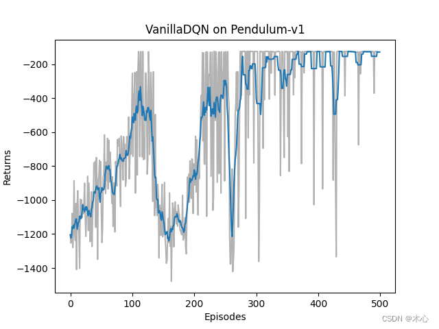
3.1 Vanilla DQN effect

The learning return of Vanilla DQN is as shown below

The maximum Q value of Vanilla DQN is estimated as shown in the figure

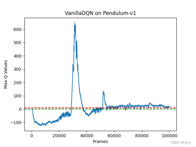
According to the analysis of the agent interaction environment, our estimate of the Q value should not exceed 0, but Vanilla DQN has exceeded 600, which is a serious overestimation problem.

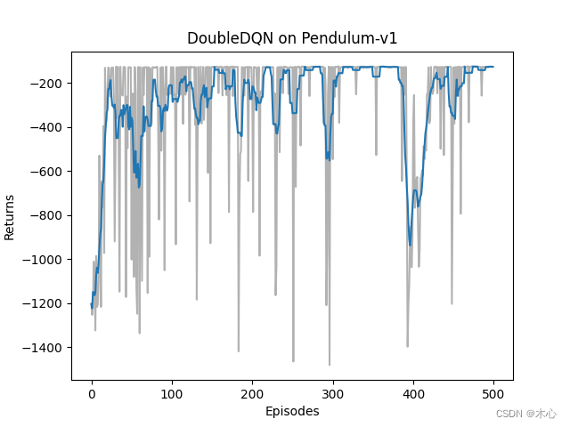
3.2 Double DQN effect

The learning return of Double DQN is as shown below

The maximum Q value of Double DQN is estimated as shown below

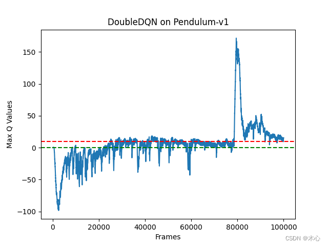
It can be seen that Double DQN does effectively alleviate the problem of overestimating the maximum Q value.

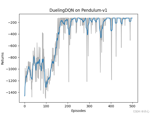
3.3 Dueling DQN effect

The learning return of Dueling DQN is as shown below

The maximum Q value of Dueling DQN is estimated as shown below

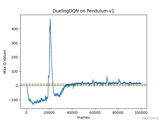
It can be seen that Dueling DQN can also alleviate the problem of overestimating the maximum Q value.

Reference

Materials
DQN及其多种变式
Hands on RL
Deep Reinforcement Learning with Double Q-learning
Reinforcement Learning with Code 【Code 1. Tabular Q-learning】
Reinforcement Learning with Code 【Chapter 7. Temporal-Difference Learning】
Reinforcement Learning with Code 【Code 4. Vanilla DQN】

Papers

• Vallina DQN

  Playing Atari with Deep Reinforcement Learning

• Double DQN

  Deep Reinforcement Learning with Double Q-learning

• Dueling DQN

  Dueling Network Architectures for Deep Reinforcement Learning