1. Signal processing - 3. Wiener filtering (including matlab code)

This article is suitable for quickly understanding Wiener filtering and being able to process actual data.

---

1. Principle of Wiener filtering

* There are many videos that explain it in detail, so I won’t go into details here. Reference is as follows:

Speech enhancement-Wiener filter 1_bilibili_bilibili

Speech enhancement-Wiener filter 2_bilibili_bilibili

2. Things to note when applying Wiener filtering

1. Wiener filtering estimates the current value of the signal based on all past observations and current observations ;                                         

2. Wiener filter is only suitable for stationary random processes ;

3. Designing a Wiener filter requires knowing the correlation function between signal and noise.

                                      

3. Wiener filter implementation

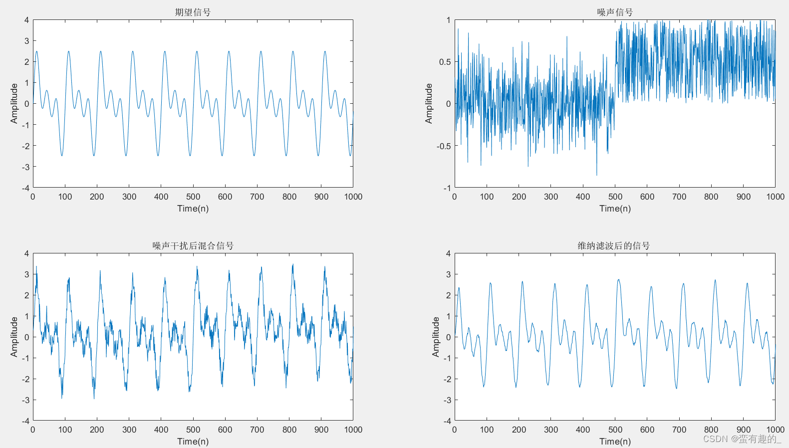
1. Construct a one-dimensional signal and mix the noise signal:

(1) Original one-dimensional signal: Signal_Original = sin(2 * pi * 10 * t) + sin(2 * pi * 20 * t) + sin(2 * pi * 30 * t)

Fs = 1000; # 采样率
N = 1000; # 采样点数
n = 0:N - 1;
t = 0:1 / Fs:1 - 1 / Fs; # 时间序列
##期望信号
Signal_Original = sin(2 * pi * 10 * t) + sin(2 * pi * 20 * t) + sin(2 * pi * 30 * t);
plot(Signal_Original)
title('期望信号');
axis([0 1000 -4 4]); # 设置坐标轴在指定的区间
xlabel('Time(n)');
ylabel('Amplitude');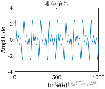

(2) Noise signal: Noise_White

##噪声信号
##前500点高斯分布白噪声，后500点均匀分布白噪声
Noise_White = [0.3 * randn(1, 500), rand(1, 500)];
plot(Noise_White)
title('噪声信号');
xlabel('Time(n)');
ylabel('Amplitude');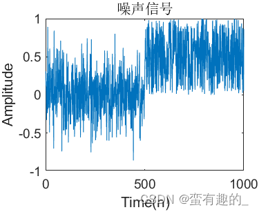

(3) Mixed signal: Signal_Original + Noise_White

##噪声干扰后信号
Mix_Signal = Signal_Original + Noise_White; # 构造的混合信号
subplot(2,2,3)
plot(Mix_Signal)
title('噪声干扰后混合信号');
axis([0 1000 -4 4]); # 设置坐标轴在指定的区间
xlabel('Time(n)');
ylabel('Amplitude');

2. Wiener filter design:

* Combined with the key points of the overall structural framework below , it will be more helpful to learn the principle of Wiener filtering~

*The main steps are as follows:

(1) The autocorrelation coefficient Rxx  of the mixed signal ( mentioned in the Wiener filtering principle ) ;

(2) The correlation coefficient Rxy  between the mixed signal and the original signal ( mentioned in the Wiener filtering principle ) ; 

xcorr function: used to calculate the correlation coefficient of two data

(3) Set the order M = 100 ( adjustable parameters, affecting the filtering effect );

(4) Construct the mixed signal autocorrelation matrix rxx(i,j) through loops ( mentioned in the Wiener filtering principle );

(5) Obtain the cross-correlation vector rxy(i) between the mixed signal and the original signal ( mentioned in the Wiener filtering principle );

(6) Obtain the designed Wiener filter coefficients ( key data, used for subsequent Wiener filtering operations on the signal ):

h = inv(rxx)*rxy'

inv function: used to find the inverse matrix; if an error occurs, the pinv function can be used to find the pseudo-inverse matrix.

##维纳滤波
Rxx = xcorr(Mix_Signal,Mix_Signal);# 得到混合信号的自相关函数
Rxy = xcorr(Mix_Signal,Signal_Original);# 得到混合信号和原始信号的互相关函数
M = 100;# 维纳滤波阶数
for i = 1:M # 得到混合信号的自相关矩阵
    for j = 1:M
        rxx(i,j) = Rxx(N-i+j);
    end
end
for i = 1:M # 得到混合信号和原信号的互相关向量
    rxy(i) = Rxy(i+N-1);
end
# 得到所要设计的Wiener滤波器系数
h = pinv(rxx)*rxy';

3. Wiener filtering of noisy signals

filter function: used to filter the signal according to the designed filter.

##维纳滤波后的信号
Signal_Filter = filter(h,1,Mix_Signal);# 将输入信号通过维纳滤波器
plot(Signal_Filter);
title('维纳滤波后的信号');
axis([0 1000 -4 4]); # 设置坐标轴在指定的区间
xlabel('Time(n)');
ylabel('Amplitude');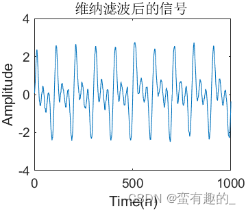

Apply the subplot function to display four pictures at the same time. The final effect is as follows:

4. Mean square error

* Mean square error is often used to evaluate the difference between signals before and after filtering

(It is more convincing to evaluate the filtering effect numerically rather than directly observing it through image display)

*Usually different evaluation indicators can be used according to different actual situations.

fprintf('引入噪声后信号相对原信号的统计均方误差:\n');
mse1 = mean((Mix_Signal-Signal_Original).^2); # 滤波后的信号相对原信号的统计均方误差
mse1
fprintf('滤波后的信号相对原信号的统计均方误差:\n');
mse2 = mean((Signal_Filter-Signal_Original).^2); # 滤波后的信号相对原信号的统计均方误差
mse2

mean function: average calculation.

* The statistical mean square error of the signal after introducing noise relative to the original signal:

mse1 = 0.2172

* Statistical mean square error of the filtered signal relative to the original signal:

mse2 = 0.0306

After applying Wiener filtering, the signal is closer to the original signal.

---