Reference: Probabilistic Diffusion Model Probabilistic Diffusion Model Theory and Detailed Interpretation of the Complete PyTorch Code
Understand the Diffusion Model from the simplest to the deeper
Article directory
Review VAE
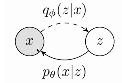
In the previous section, we learned about the principle of VAE. Generally speaking, it can be divided into two processes. One is to use q ( z ∣ x ) q(z|x)q ( z ∣ x ) gives the Encoder the process of forward learning, and the other is to usep ( x ∣ z ) p(x|z)p ( x ∣ z ) gives the Decoder the process of reverse reasoning.
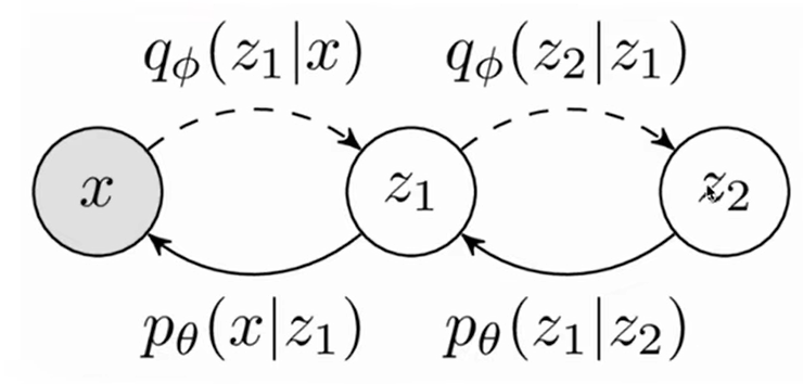
The multi-layer VAE model is actually similar to the single-layer VAE, except that on a single-layer basis, we regard it as a Markov chain, so each probability is only related to the previous probability. The above is where
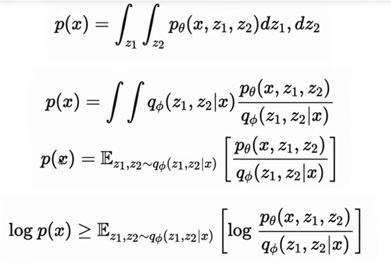
we use Jensen The confidence lower bound obtained by the inequality.
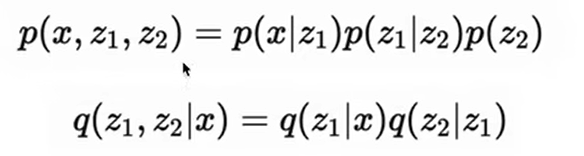
The above is the chain rule of probability (under the Markov chain). We substitute this into the maximum likelihood above, and we can get that the lower bound can be written in this form: This is the objective

function of the multi-layer VAE.
Diffusion Model
The reason why I want to introduce VAE first is because the process of multi-layer VAE is actually very similar to the Diffusion Model.

The principle of Diffusion Model is to first target x 0 x_0x0Step by step forward noise is added to obtain the final distribution x T x_TxT, and then use the process of reverse reasoning to gradually denoise, by x T x_TxTGet x 0 x_0x0。
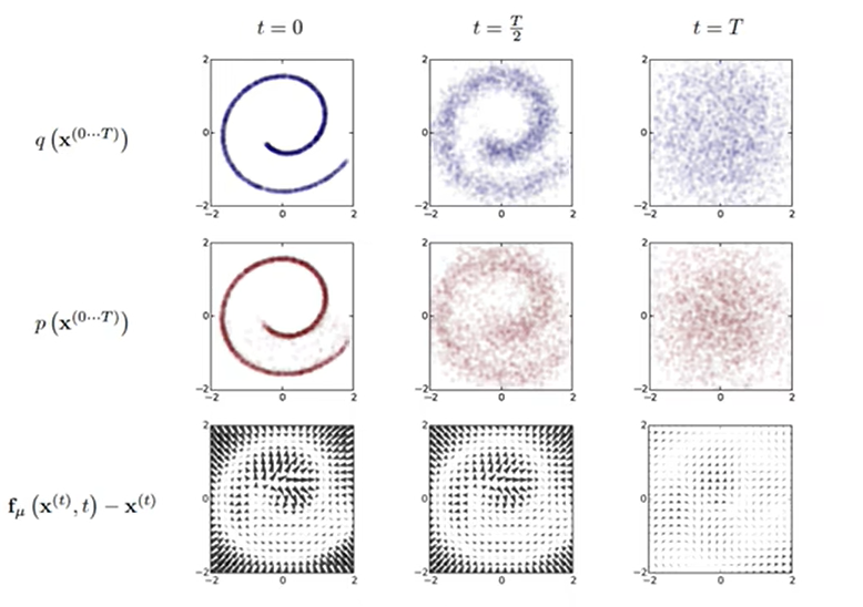
The above picture is the visualization process of Diffusion Model. In general, it is the diffusion process of adding noise (entropy increase process) q ( xt ∣ xt − 1 ) q(x_t|x_{t-1})q(xt∣xt−1) , which is the first line of the above figure, we can see that the image gradually becomes disordered as the noise is added.
For a given noise picturex T x_TxT, the Diffusion Model learned the reverse reasoning process of denoising p ( xt − 1 ∣ xt ) p(x_{t-1}|x_t)p(xt−1∣xt) , you can generate a new picture, which is the second line of the above picture. (from T time to 0 time) you can see that we have produced a new sample, which is roughly the same as the original training picture we used to add noise. are similar.
The third line is the drift amount, from which we can see the direction of image pixel movement at the previous moment and the next moment.
Diffusion process forward
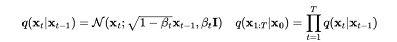
1. Given the initial data distribution x 0 ∼ q ( x ) x_0 \sim q(x)x0∼q ( x ) , Gaussian noise (affine transformation) can be continuously added to the original distribution, and the standard deviation of this noise is a fixed valueβ t \beta_tbtDetermined, the mean (expected) is at a fixed value β t \beta_tbtand current ttData at time t xt x_txtDecide. This process is a Markov chain.
2.With ttAs t continues to increase, the final data distributionx T x_TxTIt becomes a Gaussian distribution that is independent in each direction.
About xt x_txtThe algorithm that obeys the Gaussian distribution is actually the resampling technique we talked about in the previous section. We sample a zz from the normal distribution.z , then calculatex = σ z + μ x=\sigma z+\mux=σz _+μ getsxxThe sample value of x . Use resampling techniques toxt − 1 x_{t-1}xt−1You can find xt x_t by iteratingxtGaussian distribution. And q ( xt ∣ x 0 ) q(x_t|x_0)q(xt∣x0) satisfies the Markov chain.
Note: β t ∈ ( 0 , 1 ) \beta_t \in (0,1)bt∈(0,1 ) , and will grow larger over time.
3. q ( xt ) q(x_t) at any timeq(xt) derivation can also be based entirely onx 0 x_0x0and β t \beta_tbtTo calculate without iteration, the following is the calculation process:
Here we need to use the parameter renormalization technique , we let α t = 1 − β t , α ‾ t = ∏ t = 1 T α i \alpha_t=1-\beta_t,\overline \alpha_t=\displaystyle\prod^ {T}_{t=1} \alpha_iat=1−bt,at=t=1∏Tai, then change the above formula q ( xt ∣ xt − 1 ) q(x_t|x_{t-1})q(xt∣xt−1) into the resampling techniquext = σ zt − 1 + μ = β zt − 1 + 1 − β xt − 1 x_t=\sigma z_{t-1}+\mu=\sqrt{\beta}z_{t-1 }+\sqrt{1-\beta}x_{t-1}xt=σz _t−1+m=bzt−1+1−bxt−1get:
x t = α t x t − 1 + 1 − α t z t − 1 z t − 1 , z t − 2 均 . . . ∼ N ( 0 , I ) x_t=\sqrt{\alpha_t}x_{t-1}+\sqrt{1-\alpha_t}z_{t-1} ~~~~~z_{t-1},z_{t-2}均...\sim N(0,I) xt=atxt−1+1−atzt−1 zt−1,zt−2average ...∼N(0,I)
We will xt − 1 x_{t-1} in the above formulaxt−1Use about xt − 2 x_{t-2}xt−2的式子替换:
x t = α t ( α t − 1 x t − 2 + 1 − α t − 1 z t − 2 ) + 1 − α t z t − 1 = α t α t − 1 x t − 2 + α t − α t α t − 1 z t − 2 + 1 − α t z t − 1 x_t=\sqrt{\alpha_t}(\sqrt{\alpha_{t-1}}x_{t-2}+\sqrt{1-\alpha_{t-1}}z_{t-2})+\sqrt{1-\alpha_t}z_{t-1}\\ =\sqrt{\alpha_t \alpha_{t-1}}x_{t-2}+\sqrt{\alpha_t-\alpha_t\alpha_{t-1}}z_{t-2}+\sqrt{1-\alpha_t}z_{t-1} xt=at(at−1xt−2+1−at−1zt−2)+1−atzt−1=atat−1xt−2+at−atat−1zt−2+1−atzt−1
Give a basic conclusion ( independent distribution additivity ): two normal distributions X ∼ N (μ 1 , σ 1 2 ) and Y ∼ N (μ 2 , σ 2 2 ) X \sim N(\mu_1,\ sigma_1^2) and Y \sim N(\mu_2,\sigma_2^2)X∼N ( m1,p12) sum Y∼N ( m2,p22) obtained superposition distributiona X + b Y aX+bYaX+The mean of bY isa μ 1 + b μ 2 a\mu_1+b\mu_2a μ1+bμ _2,Equally a 2 σ 1 2 + b 2 σ 2 2 a^2\sigma_1^2+b^2\sigma_2^2a2 p12+b2 p22,所以 α t − α t α t − 1 z t − 2 + 1 − α t z t − 1 \sqrt{\alpha_t-\alpha_t\alpha_{t-1}}z_{t-2}+\sqrt{1-\alpha_t}z_{t-1} at−atat−1zt−2+1−atzt−1Yuz 〜 N ( 0 , I ) z \sim N(0,I)z∼N(0,I ) , so the corresponding superposition distribution mean isμ = 0 + 0 = 0 \mu=0+0=0m=0+0=0,方差 σ 2 = a 2 + b 2 = α t − α t α t − 1 + 1 − α t = 1 − α t α t − 1 , \sigma^2=a^2+b^2=\alpha_t-\alpha_t\alpha_{t-1}+1-\alpha_t=1-\alpha_t\alpha_{t-1}, p2=a2+b2=at−atat−1+1−at=1−atat−1, so substituting into the resampling formula isσ z + μ = 1 − α t α t − 1 z {\sigma}z+\mu=\sqrt{1-\alpha_t\alpha_{t-1}}zσz _+m=1−atat−1z
xt = α t α t − 1 xt − 2 + 1 − α t α t − 1 z ‾ t − 2 ( z ‾ t − 2 is a mixture of Gaussians, but still a standard normal distribution) = . . . = α ‾ tx 0 + 1 − α ‾ tz x_t=\sqrt{\alpha_t \alpha_{t-1}}x_{t-2}+\sqrt{1-\alpha_t\alpha_{t-1}}\overline z_{t -2}~~(\overline z_{t-2} is a mixed Gaussian, but still a standard normal distribution)\\ =...\\ =\sqrt{\overline\alpha_t}x_0+\sqrt{1-\ overline\alpha_t}zxt=atat−1xt−2+1−atat−1zt−2 (zt−2is a mixture of Gaussians, but still a standard normal distribution )=...=atx0+1−atz
结论:
x t = α ‾ t x 0 + 1 − α ‾ t z ( 3 ) x_t=\sqrt{\overline\alpha_t}x_0+\sqrt{1-\overline\alpha_t}z~~~~~(3) xt=atx0+1−atz (3)
Therefore, q (xt) q(x_t) at any timeq(xt) can be based onx 0 x_0x0and β t \beta_tbtto calculate without iteration:
q ( x t ∣ x 0 ) = N ( x t ; α ‾ t x 0 , ( 1 − α ‾ t ) I ) q(x_t|x_0)=N(x_t;\sqrt{\overline\alpha_t}x_0,({1-\overline\alpha_t})I) q(xt∣x0)=N(xt;atx0,(1−at) I ) , so that we can samplext x_txtThere is no need for t iterations.
So α \alphaα is more of a learning rate-like parameter, sinceβ \betaβ will become larger and larger, soα \alphaα will become smaller and smaller, so after enough momentsα → 0 , 1 − α → 1 \sqrt{\alpha} \to 0,\sqrt{1-\alpha} \to 1a→0,1−a→1 , so when time t is reached,q ( xt ∣ x 0 ) = N ( xt ; 0 , I ) q(x_t|x_0)=N(x_t;0,I)q(xt∣x0)=N(xt;0,I ) will converge to a standard normal distribution, so that we can find the maximum timettt ._ The property expressed in terms of learning rate is that ifxt x_txtPredict x 0 x_0x0, the generation in the previous stages will quickly show the bottom of the image, and the later it will be slower, the more details need to be generated.
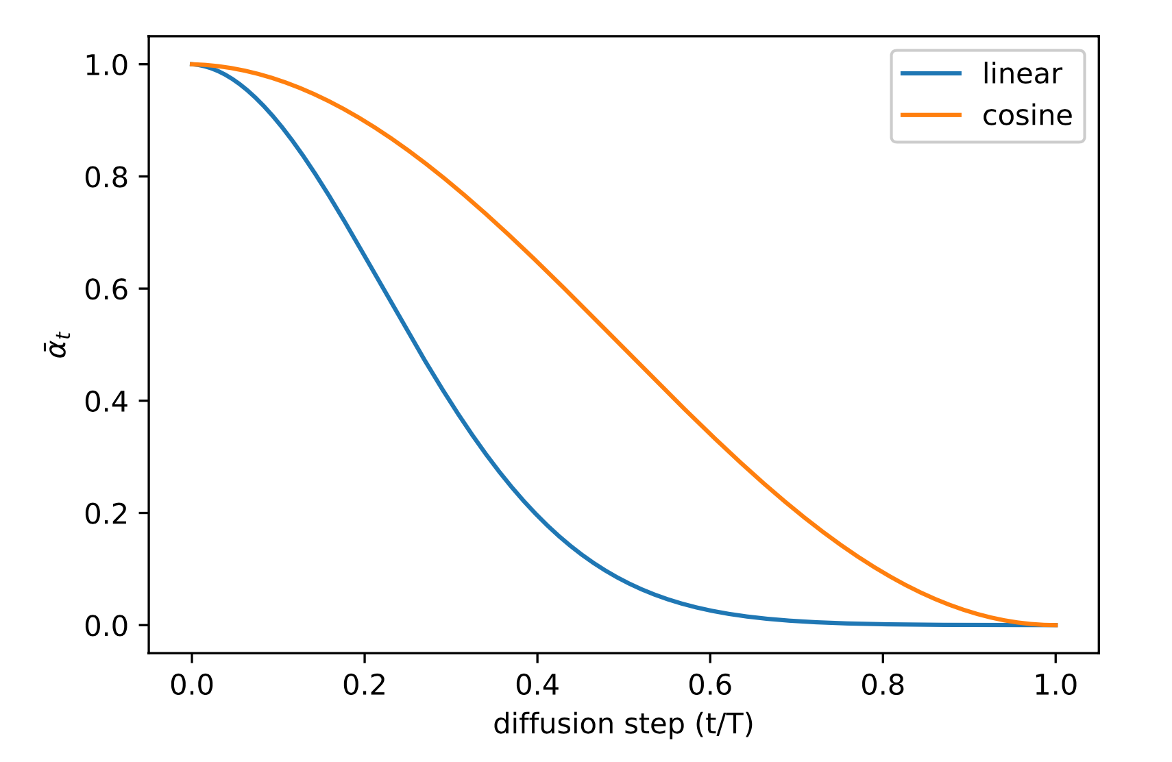
(The above figure represents α ˉ t \bar \alpha_taˉtrelationship with the diffusion step)
From here we can see some differences between Diffusion Model and VAE.
First, in VAE, the parameters are predicted through the forward and reverse process, but in diffusion, a fixed parameter is given for training. Secondly, the hidden variable zz
sampled in VAEz andxxx is related to a certain extent, and xt x_tin diffusionxtThe end result is a standard normal distribution, and xxx is irrelevant.
Also in VAExxxwazz __The dimensions of z are not necessarily the same, and in diffusionx 0 . . . . xt x_0....x_tx0....xtThe dimensions are always the same.
reverse diffusion process
If the forward process is a process of adding noise, then the reverse process is a process of denoising inference. If we can gradually obtain the reversed distribution q ( xt − 1 ∣ xt ) q(x_{t-1}|x_t )q(xt−1∣xt) , you can get from the standard normal distributionxt ∼ N ( 0 , I ) x_t \sim N(0,I)xt∼N(0,I ) Restore the original image distributionx 0 x_0x0, it is proved in Document 1 that if q ( xt − 1 ∣ xt ) q(x_{t-1}|x_t)q(xt−1∣xt) satisfies Gaussian distribution andβ t \beta_tbtSmall enough, then q ( xt − 1 ∣ xt ) q(x_{t-1}|x_t)q(xt−1∣xt) is still a Gaussian distribution, if xt . . . x 0 x_t...x_0is graduallyxt...x0It is really difficult to calculate by fitting to find the Gaussian distribution parameters it obeys. So we need to construct a parameter distribution for estimation, and the reverse diffusion process is still a Markov chain.
We use a deep learning model (parameters are θ \thetaθ , the current mainstream is the structure of U-Net+attention) to predict such an inverse distributionp θ p_\thetapi. (Similar to VAE):
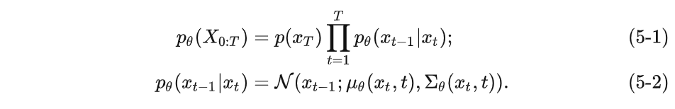
Although we cannot get the reversed distribution q ( xt − 1 ∣ xt ) q(x_{t-1}|x_t)q(xt−1∣xt) , but if we knowx 0 x_0x0, can be calculated by the following formula:
q ( x t − 1 ∣ x t , x 0 ) = N ( x t − 1 ; μ ~ ( x t , x 0 ) , β ~ t I ) ( 6 ) q(x_{t-1}|x_t,x_0)=N(x_{t-1};\tilde\mu(x_t,x_0),\tilde\beta_tI)~~~~(6) q(xt−1∣xt,x0)=N(xt−1;m~(xt,x0),b~tI) (6)
The reasoning is as follows:
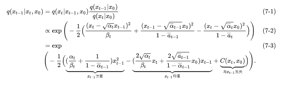
We use Bayes’ formula to reason about (7-1):
q ( a ∣ b , c ) = q ( a , b , c ) q ( b , c ) q(a|b,c)=\frac{q (a,b,c)}{q(b,c)}q(a∣b,c)=q(b,c)q(a,b,c)
Among them, the chain rule q ( a , b , c ) = q ( b ∣ a , c ) q ( a ∣ c ) q ( c ) q(a,b,c)=q(b|a,c)q( a|c)q(c)q(a,b,c)=q(b∣a,c)q(a∣c)q(c), q ( b , c ) = q ( b ∣ c ) q ( c ) q(b,c)=q(b|c)q(c) q(b,c)=q ( b ∣ c ) q ( c )
Therefore, substitute the original formula= q ( b ∣ a , c ) q ( a ∣ c ) q ( c ) q ( b ∣ c ) q ( c ) = q ( b ∣ a , c ) q ( a ∣ c ) q ( b ∣ c ) =\frac{q(b|a,c)q(a|c)q(c)}{q(b|c)q(c)}= \frac{q(b|a,c)q(a|c)}{q(b|c)}=q(b∣c)q(c)q(b∣a,c)q(a∣c)q(c)=q(b∣c)q(b∣a,c)q(a∣c), since it is a Markov chain, the above formula is also equivalent to q ( b ∣ c ) q ( a ∣ c ) q ( b ∣ c ) q(b|c)\frac{q(a|c)}{q (b|c)}q(b∣c)q(b∣c)q(a∣c)
We can see that in equation (7-1), we use Bayes' formula to transform this reverse process into a forward process, and (7-2) is its corresponding Gaussian distribution probability density function. We expand it to get formula (7-3), where xt − 1 x_{t-1}xt−1Irrelevant terms include only xt & x 0 x_t \& x_0xt&x0The items are classified into C ( xt , x 0 ) C(x_t,x_0)C(xt,x0)
( The probability density function of the Gaussian distribution is f ( x ) = 1 2 π σ e − ( x − μ ) 2 2 σ 2 f(x)=\frac{1}{\sqrt{2\pi}\sigma}e ^{-\frac{(x-\mu)^2}{2\sigma^2}}f(x)=2 p.mp1e−2 p2( x − μ )2)
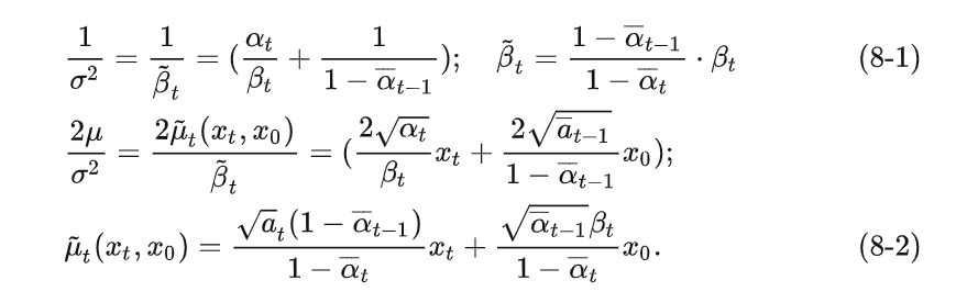
We said before that q ( xt − 1 | xt ) q(x_{t-1}|x_t)q(xt−1∣xt) is still a Gaussian distribution, which means that the above formula can be organized into the formula of a Gaussian distribution, and the corresponding exponential part of the general Gaussian probability density function isexp ( − ( x − μ ) 2 2 σ 2 ) = exp ( − 1 2 ( 1 σ 2 x 2 − 2 μ σ 2 x + μ 2 σ 2 ) ) exp(-\frac{(x-\mu)^2}{2\sigma^2})=exp(-\frac {1}{2}(\frac{1}{\sigma^2}x^2-\frac{2\mu}{\sigma^2}x+\frac{\mu^2}{\sigma^2} ))exp(−2 p2( x − μ )2)=exp(−21(p21x2−p22 mx+p2m2)) , which corresponds to the form compiled in (7-3), therefore:
Use the β \beta mentioned in the forward directionβ replaces the varianceσ 2 \sigma^2p2 , get:
Due to the inference 3 mentioned in the diffusion process, we know that xt x_t at any timextCan be determined by x 0 x_0x0and β \betaβ means. therefore:
x 0 = 1 α ˉ t ( x t − β t 1 − α ˉ t z ˉ t ) x_0=\frac{1}{\sqrt{\bar\alpha_t}}(x_t-\frac{\beta_t}{\sqrt{1-\bar\alpha_t}}\bar z_t)~~~ x0=aˉt1(xt−1−aˉtbtzˉt) ( x t x_t xt(formula deformation)
Substituting this into (8-2) we get
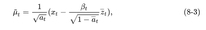
The Gaussian distribution z ˉ t \bar z_tzˉtThe noise predicted by the depth model (used for denoising) can be viewed as z θ ( xt , t ) , z_\theta(x_t,t),zi(xt,t ) , get:
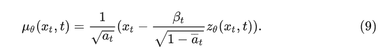
After a series of calculations, we first get q ( xt − 1 ∣ xt ) q(x_{t-1}|x_t)q(xt−1∣xt) of the Gaussian distribution probability density function, and then organize it into the general form of the exponential part of the Gaussian distribution, thereby obtaining the corresponding mean and variance, where the varianceβ \betaβ is a constant value, and the meanμ \muμ is then expressed asxt, t x_t,txt,t is the function form of the parameter
In this way, the inference of each step of DDPM can be summarized as:
1) Each time step passes xt x_txtandtt _t to predict Gaussian noisez θ ( xt , t ) z_\theta(x_t,t)zi(xt,t ) , and then the meanμ θ ( xt , t ) \mu_\theta(x_t,t)mi(xt,t)
2) Get the variance Σ θ ( xt , t ) \Sigma_\theta(x_t,t)Si(xt,t),DDPM中使用untrained Σ θ ( x t , t ) = β ~ t \Sigma_\theta(x_t,t)=\tilde \beta_t Si(xt,t)=b~t(That is, the training variance is not used as a fixed parameter), and it is considered that β ~ t = β t \tilde \beta_t=\beta_tb~t=bt和 β ~ t = 1 − α ˉ t − 1 1 − α ˉ t ⋅ β t \tilde \beta_t=\frac{1-\bar \alpha_{t-1}}{1-\bar \alpha_t} \cdot \beta_t b~t=1−aˉt1−aˉt−1⋅btApproximate results
3) According to (5-2), we get q ( xt − 1 ∣ xt ) q(x_{t-1}|x_t)q(xt−1∣xt),利用重参数技巧得到 x t − 1 x_{t-1} xt−1
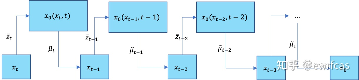
重复上述步骤逐步去噪,直到计算出 x 0 x_0 x0,去噪过程完毕。
Diffusion训练
讲完了前向加噪的扩散过程和逆向去噪的推断过程(虽然文字上来看原理很简单,但是公式好繁杂)。现在我们讲讲如何训练diffusion model以得到靠谱的参数 μ θ ( x t , t ) 和 Σ θ ( x t , t ) \mu_\theta(x_t,t)和\Sigma_\theta(x_t,t) μθ(xt,t)和Σθ(xt,t),方法还是最大对数似然(此处用的最小化负对数似然)。
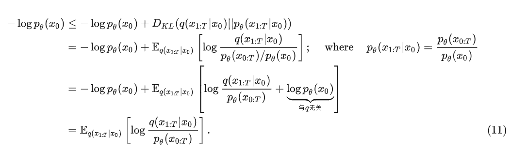
由于整个Diffusion模型和VAE很相似,训练过程也是,由于KL散度恒大于0,因此我们在负对数似然上加上一个KL散度就构成了它的上界(和VAE最大对数似然的时候正好相反,那时是减去一个KL散度是下界):
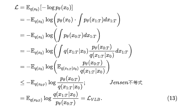
利用詹森不等式,我们就能得到(这块看的不太细,记住结论就好):
我们进一步对 L V L B L_{VLB} LVLB进行推导,可以得到熵与多个KL散度的累加2,其中分母是扩散过程,分子是逆扩散过程:
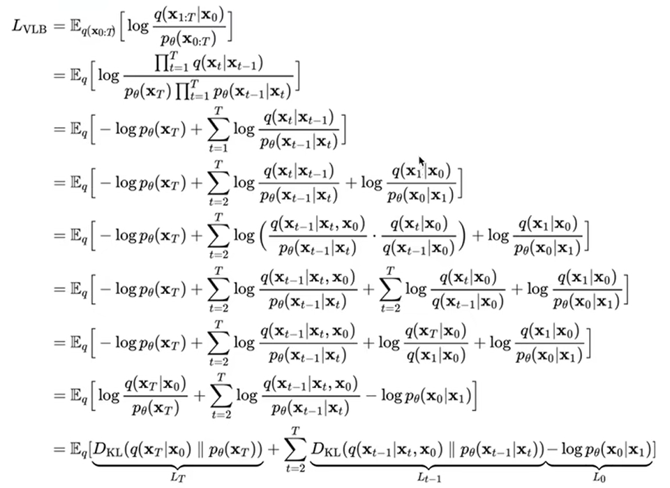
(上式【从 L V L B L_{VLB} LVLB开始为第一行】第四行到第五行又是应用了贝叶斯公式,先逆向马尔科夫链补上了一个 x 0 x_0 x0再应用了和之前前向中讲到的一模一样的贝叶斯公式)
第六行的第三项 ∑ t = 2 T l o g q ( x t ∣ x 0 ) q ( x t − 1 ∣ x 0 ) \sum^T_{t=2}log\frac{q(x_t|x_0)}{q(x_{t-1}|x_0)} ∑t=2Tlogq(xt−1∣x0)q(xt∣x0)可化简,最后与第四项以及第一项可合并,最终得到了第七行的式子
最后一行将其简化为了含有KL散度的式子,其中 L T L_T LT不含参(q分布不含参, x T x_T xT逆向过程最终为纯高斯噪声)相当于常量可以直接忽略, L t − 1 L_{t-1} Lt−1是逆扩散过程的KL散度,最后考虑的还是 L t − 1 和 L 0 L_{t-1}和L_0 Lt−1和L0。
并且由于 q 和 p θ q和p_{\theta} q和pθ其实都是高斯分布,并且 q q q是关于参数 β t \beta_t βt的高斯分布,且 β t \beta_t βt是untrained的固定参数(忘记的,点此回去), p θ p_{\theta} pθ的高斯分布均值是 μ θ \mu_{\theta} μθ,方差是 Σ θ \Sigma_\theta Σθ且 Σ θ \Sigma_\theta Σθ也是untrained的固定参数。因此可训练的参数 θ \theta θ只在 p θ p_\theta pθ中。
上面刚才推导的式子也可写为:

给出一个结论:对于两个高斯分布p,q而言,它们的KL散度可等价为
D K L ( p , q ) = l o g σ 2 σ 1 + σ 1 2 + ( μ 1 − μ 2 ) 2 2 σ 2 2 − 1 2 D_{KL}(p,q)=log\frac{\sigma_2}{\sigma_1}+\frac{\sigma_1^2+(\mu_1-\mu_2)^2}{2\sigma_2^2}-\frac{1}{2} DKL(p,q)=logσ1σ2+2σ22σ12+(μ1−μ2)2−21
让我们把 L t − 1 L_{t-1} Lt−1的式子用上式表示出来,得到:
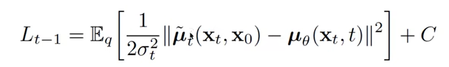
(此处 L t − 1 L_{t-1} Lt−1应该是笔误,实为 L t L_t Lt, L V L B L_{VLB} LVLB给出的是 t = 2 t=2 t=2开始,在(14-3)中已经被改为 t = 1 t=1 t=1开始到 T − 1 T-1 T−1)
然后将 μ ~ t \tilde \mu_t μ~t用(8-2)替换, μ θ \mu_\theta μθ用(9)替换, x t x_t xt用(3)替换,得到:
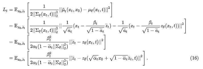
从(16)可以看出,diffusion训练的核心就是取学习高斯噪声 z ˉ t , z θ \bar z_t,z_\theta zˉt,zθ之间的均方误差MSE。论文中作者说我们可以将(16)式子中前面的这个系数给直接丢掉,这样训练会更稳定。
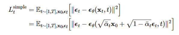
最后论文给出的式子,我们将 z ˉ t \bar z_t zˉt替换为 ϵ \epsilon ϵ, z θ z_\theta zθ替换为 ϵ θ \epsilon_\theta ϵθ,DDPM将loss进一步简化为:
训练过程可以看做:
1)获取输入 x 0 x_0 x0,从1…T随机采样一个 t t t
2) 从标准高斯分布采样一个噪声 ϵ ∼ N ( 0 , I ) \epsilon \sim N(0,I) ϵ∼N(0,I)
3) 最小化loss函数
总结
最后我们给出DDPM提供的训练/测试(采样)流程图
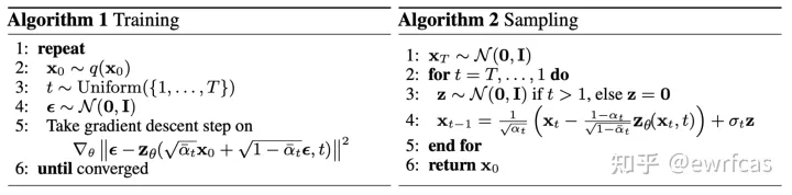
在训练过程中,我们要输入 x 0 x_0 x0进行随机采样时刻 t t t并采样噪声 ϵ \epsilon ϵ,然后对loss函数进行梯度下降直到拟合。而在测试采样过程中,我们则利用马尔科夫链逆向逐步去噪计算 x T x_T xT直到 x 0 x_0 x0作为最后的生成结果。
加速Diffusion采样和方差的选择(DDIM)
通过遵循反向扩散过程的马尔可夫链从DDPM生成样品非常慢,因为高质量生成需要的 T T T最多要走一千步或是几千步。“例如,从 DDPM 采样大小为 20 × 50 的 32k 图像大约需要 32 小时,但从 Nvidia 2080 Ti GPU 上的 GAN 采样不到一分钟。”
这就导致diffusion的前向过程非常缓慢。在denoising diffusion implicit model (DDIM)中提出了一种牺牲多样性来换取更快推断的手段。
一种简单的方法是运行一个跨步的采样,通过每隔 ⌈ T / S ⌉ \lceil T/S \rceil ⌈T/S⌉步进行采样更新,总共采样 S S S步,这样就能有效减少采样数量。
另一种方法是重写 q σ ( x t − 1 ∣ x t , x 0 ) q_\sigma(x_{t-1}|x_t,x_0) qσ(xt−1∣xt,x0)的标准差 σ t \sigma_t σt:
根据(3)我们可知:
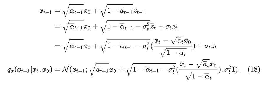
(第二步利用了独立高斯分布可加性)
最终得到的(18)将方差 σ t 2 \sigma_t^2 σt2迎入到了均值中,当 σ t 2 = β ~ t = 1 − α ˉ t − 1 1 − α ˉ t \sigma_t^2=\tilde \beta_t=\frac{1-\bar \alpha_{t-1}}{1-\bar \alpha_t} σt2=β~t=1−αˉt1−αˉt−1时,(18)等价于(6)。我们给定一个 η \eta η作为控制采样随机性的超参数 σ t 2 = η β ~ t \sigma_t^2=\eta \tilde \beta_t σt2=ηβ~t(作用类似于调整方差的大小),当 η = 1 \eta=1 η=1的时候就等价于DDPM,当 η = 0 \eta=0 η=0的时候是DDIM
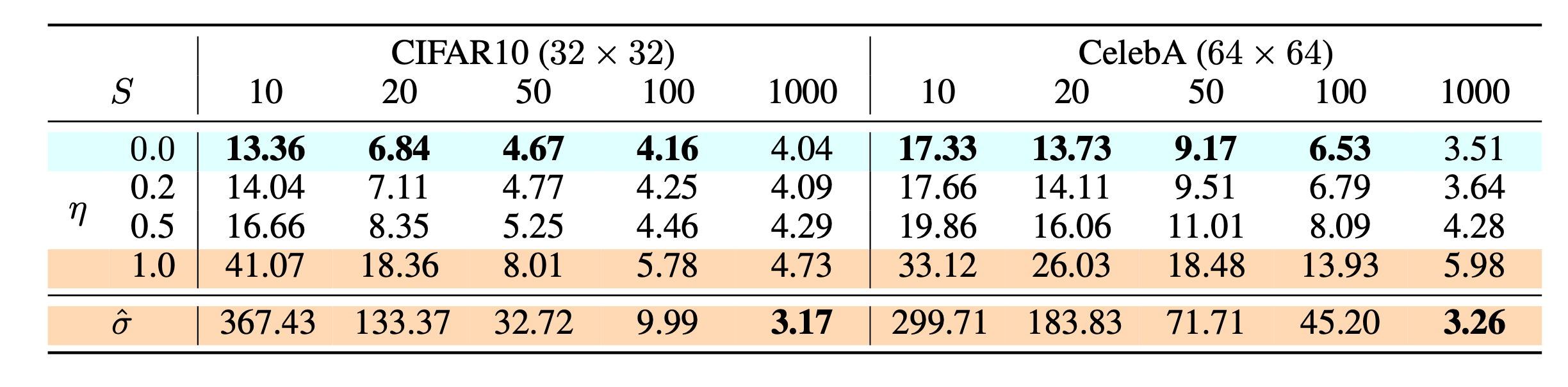
(上图是不同设置的扩散模型在 CIFAR10 和 CelebA 数据集上的 FID 得分,包括了DDIM( η = 0 \eta=0 η=0)以及DDIM( σ ^ \hat \sigma σ^)( η = 1 \eta=1 η=1))
根据上表可知,数据量较小时DDIM的训练更快,而数据量较大时使用DDPM并采用更大的方差效果更好
与DDPM相比,DDIM能够:
1.使用更少的步骤生成更高质量的样本。
2.具有“一致性”属性,因为生成过程是确定性的,这意味着以同一潜在变量为条件的多个样本应该具有类似的高级特征。
3.由于一致性,DDIM 可以在潜在变量中执行语义上有意义的插值。
Feller, William. “On the theory of stochastic processes, with particular reference to applications.” Proceedings of the [First] Berkeley Symposium on Mathematical Statistics and Probability. University of California Press, 1949. ↩︎
Feller, William. “On the theory of stochastic processes, with particular reference to applications.” Proceedings of the [First] Berkeley Symposium on Mathematical Statistics and Probability. University of California Press, 1949. ↩︎