Forgetting factor recursive least squares parameter estimation (FFRLS)

Battery parameter identification based on least squares method based on forgetting factor

The least squares method is the most commonly used estimation method in system identification. In order to overcome the "data saturation" problem of the least squares method, we usually use the Forgetting Factor Recursive Least Square (FFRLS) algorithm containing a forgetting factor to identify the parameters of the battery model.

1. Establishment of second-order RC mathematical model

Generally speaking, we need to consider the following points to establish an accurate battery model: the model can accurately describe the dynamic and static characteristics of the battery; the model is low in complexity and easy to calculate; the engineering implementation of the model is relatively simple and feasible. Taking comprehensive considerations into account, we choose the second-order RC equivalent circuit model. In order to identify the parameters of the battery equivalent circuit model, we need to transform the battery model into a mathematical form that can be identified using the least squares method. For specific recursion formulas, please refer to battery SOC related literature.

2. Identification of forgetting factors by recursive least squares method

System parameters

Qn = 2.59*3600;
ff = 1;
N = length(Ut);     % 数据长度
dt=1;               % 【数据采样间隔】

Calculation of SOC experimental data

ocv = nan(1,N);
soc_act(1)=1;
ocv(1)=Ut(1);
for i=2:N
    soc_act(i)=soc_act(i-1)-I(i)/(Qn);
    nihe=[1.936,-7.108,9.204,-4.603,1.33,3.416];
    ocv(i)=polyval(nihe,soc_act(i)); 
end

FFRLS parameter online identification algorithm

function [R0,R1,R2,C1,C2] = FFRLS(Ut,I,Qn,P,ff,cs0)

N = length(Ut);      %数据长度

%SOC计算与OCV计算
soc = nan(1,N);
ocv = nan(1,N);
soc(1)=1;
ocv(1)=Ut(1);
for i=2:N
    soc(i)=soc(i-1)-I(i)/(Qn);
    ocv(i)=polyval(P,soc(i)); 
end

ev = zeros(1,N); 
for i=1:N
    ev(i)=ocv(i)-Ut(i);
end

%%%2.RLS递推最小二乘辨识
% cs0=[   1.2761;
%        -0.2899;
%         0.0365;
%        -0.0449;
%         0.0095];

% cs0=[ 1.1414;
%    -0.1640;
%     0.0709;
%    -0.0796;
%     0.0109];


p0=10^(-1)*eye(5,5);
cs=[cs0,cs0,zeros(5,N-1)];        %被辨识参数矩阵的初始值及大小
e=zeros(5,N);               %相对误差的初始值及大小
error1 = zeros(1,N);
%%%%2.2计算增益矩阵以及求辨识参数
for k=3:N                  %开始求K 
    h1=[ev(k-1),ev(k-2),I(k),I(k-1),I(k-2)]';
    q=h1'*p0*h1+ff;           %遗忘因子
    k1=p0*h1/q;              %求出K(k)的值
    error1(k)=ev(k)-h1'*cs0;  %求电压实验值和理论值误差
    cs1=cs0+k1*error1(k);
    e1=cs1-cs0;               %求参数当前值与上一次的值的差值
    e2=e1./cs0 ;              %求参数的相对变化
    e(:,k)=e2;                %把当前相对变化的列向量加入误差矩阵的最后一列       
    cs0=cs1;                  %新获得的参数作为下一次递推的旧参数
    cs(:,k)=cs1;              %把辨识参数c 列向量加入辨识参数矩阵的最后一列 
    p1=(p0-k1*h1'*p0)/ff;     %求出 p(k)的值
    p0=p1;                    %递推
end                           %大循环结束


%%%3.分离参数
a1=cs(1,1:N); a2=cs(2,1:N); a3=cs(3,1:N); a4=cs(4,1:N); a5=cs(5,1:N);
%==========================输出结果============================= 
a0=1./(1-a1-a2);
R0=-a5./a2;
b1=-a2.*a0;
b2=a0.*(a1+2.*a2);
b3=a0.*(a3+a4+a5);
b4=-a0.*(a4+2.*a5);
dd=b2.*b2-4.*b1;
tt=[(b2+sqrt(dd))/2;(b2-sqrt(dd))/2];
t2=abs(tt(1,:));
t1=abs(tt(2,:));
R2=(t2.*b3+t1.*R0-b4)./(t2-t1);
R1=abs(b3-R0-R2);
C1=t1./R1;
C2=t2./R2;

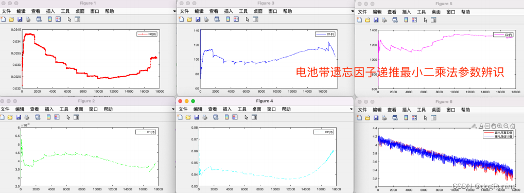
3. Identification results

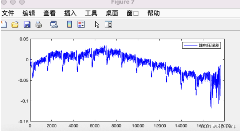
Terminal voltage error

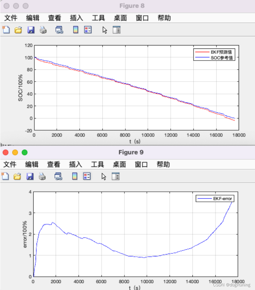
SOC estimate&& SOC error