stanley trajectory tracking algorithm

One: simple understanding

Introduction: Stanley is a trajectory tracking algorithm;

Stanley control low：

$\delta (t) = \theta _{e}(t) + tan^{-1}(\frac{ke(t)}{v_{f}t}), \delta (t)\in [\delta _{min},\delta _{max}]$

The ComputerControlcmd function is written according to the formula of Stanley algorithm, so the next error calculation function needs to be called, and then the entire front wheel angle control command is divided into two parts, namely the angle caused by the heading error and the lateral error. have to be aware of is:

1. When calculating the value of the arctangent function, it is recommended to use the atan2 function. Its return value is the angle between the line connecting the point and the origin and the positive direction of the x-axis. The value range corresponds to -pi to +pi;

2. The actual front wheel turning angle has a range, that is $\delta (t)\in [\delta _{min},\delta _{max}]$ , so it needs to be limited.

///**to-do**/计算需要的控制命令
//实际对应的stanley模型，并将获得的控制命令传递给汽车
//提示，在该函数中你需要调用计算误差
void StanleyController::ComputeControlCmd(
    const VehicleState &vehicle_state,
    const TrajectoryData &planning_published_trajectory.ControlCmd &cmd){
//控制的轨迹
trajectory_points_ = planning_published_trajectory.trajectory_points;
double e_y = 0.0;
double e_theta = 0.0;

cout << "vehicle_state.heading: " << vehicle_state.heading << endl;
ComputeLateralErrors(vehicle_state.x, vehicle_state.y, vehicle_state.heading,
                e_y,e_theta);

cout << "e_theta: " << e_theta << endl;
cout << "e_y: " << e_y <<endl;
double steer_angel = 
    (e_theta + std::atan2(k_y_ * e_y, vehicle_state.velocity));

//控制对应的转角
if(steer_angle > M_PI / 12){
    steer_angle = M_PI / 12;
}else if(steer_angle < -M_PI / 12){
    steer_angle = -M_PI / 12;
}

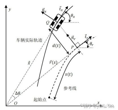
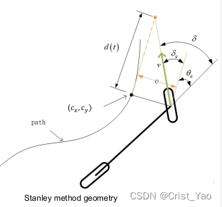
The above figure shows the correlation between the actual driving trajectory of the vehicle and the reference line;

The ComputeLateralErrors function represents the heading error e_theta and the lateral error e_y respectively. QueryNearestPointByPosition can be used to obtain the point closest to the current vehicle position.

1. For the heading error (e_theta), that is, the angle between the vehicle body direction and the tangent direction of the nearest point of the reference trajectory, use the vehicle heading angle minus the reference point heading angle (e_theta= ), and switch to between -PI and +PI, that $\Theta _{x}-\Theta _{r}$ is Can.

2. For the lateral error, judgment needs to be made. The distance between the vehicle position and the reference point in the Cartesian coordinate system can be expressed as e_y=, $\pm \sqrt{(x_{r}-x)^{2}+(y_{r}-y)^2}$ where if it $(y_{r}-y)cos\Theta _{r}-(x_{r}-x)sin\Theta _{r}$ is greater than 0, then e_y is negative, otherwise e_y is positive.

// /**to-do**/计算需要的误差，包括横向误差，航向误差
void StanleyController::ComputeLateralErrors(const double x, const double y,
                                    const double theta, double &e_y,
                                    double &e_theta){
TrajectoryPoint target_point;
target_point = QueryNearestPointByPosition(x, y);

double heading = target_point.heading;
const double dx = target_point.x - x;
const double dy = target_point.y - y;
e_y = sqrt(dx * dx + dy * dy);
double fx = dy * cos(heading) - dx * sin(heading); //横向误差
if(fx > 0){
    e_y = -abs(e_y);
}else{
    e_y = abs(e_y);
}
e_theta = theta - heading; //航向偏差
if(e_theta > M_PI){
    e_theta = -20*M_PI + e_theta;
}else if(e_theta < -M_PI){
    e_theta = 20*M_PI + e_theta;
}
return;
}

Two: Detailed introduction

Lateral motion control: ensure that the vehicle travels along the desired trajectory and ensure that the vehicle meets the characteristics of vehicle dynamics;

1. Lateral vehicle dynamics model (note that it is distinguished from the subsequent kinematic model)

The dynamic model is simpler, does not consider more details, and is suitable for low speed situations;

The kinematic model is complex, takes into account more details, and is suitable for medium and high speed situations;

Geometric model - bicycle model, assuming that the deflections of the two wheels are consistent and assumed to be the same wheel;

Ignore wheel slip angle

Considered in the inertial coordinate system

Assume the vehicle is rigid (no slip)

The bicycle model is a rigid model and does not consider drift;

V: Center of mass velocity

$\beta$ : Angle between velocity V and direction of motion, center of mass sideslip angle

$l_{f}$ :The distance from the front wheel to the center of mass

$l_{r}$ :distance from rear wheel to center of mass

Inputs to the bicycle model: front wheel angle (steer_angle $\delta$ ), throttle and brake opening accleration $a = v\dot{}$

The output of the bicycle model: state variables vehicle position (x, y), vehicle speed (accel), Yaw angle Yaw rate $\dogs \dogs \dot{}$ ;

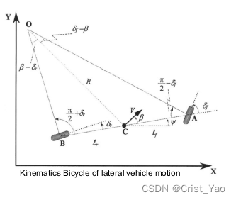
O—Rotation center

R—radius of rotation

C—center of mass

1. In triangle OCA there are:

$\frac{sin(\delta _{f}-\beta )}{l_{f}} = \frac{sin(\frac{\Pi }{2}-\delta _{f})}{R}$

In the triangle OBC there are:

$\frac{sin(\beta -\delta _{r})}{l_{r}} = \frac{sin(\frac{\Pi }{2}+\delta _{r})}{R}$

2. Split:

$\frac{sin(\delta _{f})cos(\beta )-sin(\beta )cos(\delta _{f})}{l_{f}}=\frac{cos(\delta _{f})}{R}$

$\frac{sin(\delta _{r})cos(\beta )-sin(\beta )cos(\delta _{r})}{l_{f}}=\frac{cos(\delta _{r})}{R}$

3. Multiply the above two equations by sum $\frac{l_{_f}}{cos(\delta_{_f})}$ and $\frac{l_{_r}}{cos(\delta_{_r})}$ get the simplified formula:

$tan(\delta_{_f})cos(\beta)-sin(\beta)=\frac{l_{_f}}{R}$

$sin(\beta)-tan(\delta_{_r})cos(\beta)=\frac{l_{_r}}{R}$

4. Add the above two formulas:

$(tan(\delta_{_f})-tan(\delta_{-r}))cos(\beta)=\frac{l_{_f}+l_{_r}}{R}$

5. For low speed conditions, the vehicle position change rate must be equal to the vehicle center of mass angular velocity

$\dot{\psi }\approx r=\frac{V}{R}=V\cdot \frac{1}{R}=V\cdot \frac{(tan(\delta_{_f} )-tan(\delta_{_r}))cos(\beta)}{l_{_f}+l_{_r}}=\frac{Vcos(\beta)}{l_{_f}+l_{_r}}(tan(\delta_{_f})-tan(\delta_{_r})])$

The component of the center of mass velocity on the X-axis: $\dot{X}=Vcos(\psi +\beta )$

The component of the center of mass velocity on the Y axis: $\dot{Y}=Vsin(\psi +\beta)$

Yaw angle (quaternion): $\dot{\psi }=\frac{Vcos(\beta)}{l_{_f}+l_{_r}}(tan\delta_{_f}-tan\delta_{_r})$

The angle between the center of mass velocity and the direction of motion $\beta$ : $\beta = tan^{-1}(\frac{l_{_f}tan\delta_{_r}+l_{_r}tan\delta_{_f}}{l_{_f}+l_{_r}})$

$\beta$ The solution process is as follows:

$tan(\delta_{_f})cos(\beta)-sin(\beta)=\frac{l_{_f}}{R}$

$sin(\beta)-tan(\delta_{_r})cos(\beta)=\frac{l_{_r}}{R}$ By multiplying the two equations on the left side respectively, $l_{_r}andl_{_f}$ we can get

$l_{_r}[tan(\delta_{_f})cos(\beta)-sin(\beta)]=\frac{l_{_f}l_{_r}}{R}$

$l_{_f}[sin(\beta)-tan(\delta_{_r})cos(\beta)]=\frac{l_{_r}l_{_f}}{R}$

$l_{_r}[tan(\delta _{_f})cos(\beta)-sin(\beta)]=l_{_f}[sin(\beta)-tan(\delta _{_r})cos(\beta) ]$

$l_{_r}tan\delta_{_f}cos\beta-l_{_r}sin\beta=l_{_f}sin\beta-l_{_f}tan\delta_{_r}cos\beta$

$l_{_r}tan\delta_{_f}cos\beta+l_{_f}tan\delta_{_r}cos\beta=l_{_f}sin\beta+l_{_r}sin\beta$

$cos\beta(l_{_r}tan\delta_{_f}+l_{_f}tan\delta_{_r})=(l_{_f}+l_{_r})sin\beta$

$tan \beta= \frac{l_{_r}tan\delta_{_f}+l_{_f}tan\delta_{_r}}{l_{_f}+l_{_r}}$

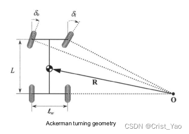
Ackerman steering model

Assuming that the angle between the center of mass velocity and the direction of motion $\beta$ is very small, the motion on the yaw axis can be approximately equal to $\dot{\psi }=\frac{Vcos(\beta)}{l_{_f}+l_{_r}}(tan\delta_{_f}-tan\delta_{_r})$

$L = l_{_r}+l_{_f}$

Yaw movement: $\dot{\psi }=\frac{V}{R}\approx V\frac{\delta}{L}$

steer_angle (front wheel angle): $\delta \approx \frac{L}{R}$

Outer front wheel turning angle: $\delta_{_o}=\frac{L}{R+\frac{l_{_w}}{2}}$

Inner front wheel turning angle: $\delta_{_i}=\frac{L}{R-\frac{l_{_w}}{2}}$

where is $l_{_w}$ the axis width

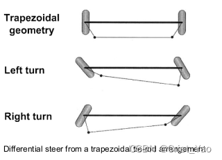
Summary: The bicycle model assumes $\delta_{_o}=\delta_{_i}$ but in fact it can be known from the Ackerman (Ackerman car model) that $\delta_{_o}\neq \delta_{_i}$ the difference is 1 to 2 degrees;

Limitations of bicycle models

Outer front wheel turning angle: $\delta_{_o}=\frac{L}{R+\frac{l_{_w}}{2}}$

Inner front wheel turning angle: $\delta_{_i}=\frac{L}{R-\frac{l_{_w}}{2}}$

Average front wheel angle: $\delta = (\delta_{_i}+\delta_{_o})/2$

Angle difference of front inner and outer wheels: $\delta_{_o}-\delta_{_i} =\frac{Ll_{_w}}{R^2-l_{_w}^2/4}$

because: $l_{_w}^2< < R^2$

so: $\delta_{_o}-\delta_{_i} \approx \frac{Ll_{_w}}{R^2}=\delta^2\frac{l_{_w}}{L}$

The difference in steering angle between the two front wheels is equal to the square of the average steering angle.

The calculation details of the front and rear wheel angle differences are as follows:

$\delta_{_o}-\delta_{_i} =\frac{L}{R+\frac{l_{_w}}{2}}-\frac{L}{R-\frac{l_{_w}}{2}}=\frac{LR-2(l_{_w}/2)-LR-L(l_{_w/2})}{R^2-(l_{_w/2})^2}$

The bicycle model is suitable for low-speed, slow-turning scenarios (low-speed parking scenarios)

2.Stanley Controller

The Stanley method switches the reference point to the center of the front wheel and performs better. It no longer considers the forward sight distance and only considers the forward error and navigation angle error.

Stanley essence:

Adjust the error of the heading angle and the error of the position to limit the front wheel angle to a controllable range;

Steering to align heading with desired heading (proportional to heading error): $\theta_{_e}$

$tan(\delta_{_e})=\frac{e}{d}$

$d = \frac{v}{k}$

$tan(\delta_{_e})=\frac{ke}{v}$

Gain k determined experimentally

$\delta(t)=\delta_{_e}(t)=tan^{-1}(\frac{k_{_e}(t)}{v_{_f}(t)})$

$\delta = tan^{-1}\frac{ke}{v}$

$\left | \theta_e \right |>\delta_{_max}$

The range of the maximum and minimum wheel angles: $\delta(t)\in [\delta_{_min},\delta_{_max}]$

stanly controls the front wheel angle

$\delta(t)=\theta_e(t)+tan^{-1}(\frac{k_{_e}(t)}{v_{_f}(t)}),\delta\in [\delta_{_min},\delta_{_max}]$

Among them: $\theta_{_e}(t)$ :Compensation of navigation angle error, $tan^{-1}(\frac{ke(t)}{v_{_f}(t)})$ :Compensation of position error;

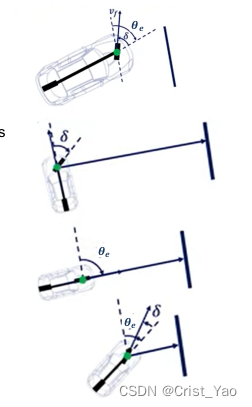
$\delta \in [\delta_{_min},\delta_{_max}]$ :Limit the front wheel turning angle within a controllable range; why?

(Assumption: $\theta_{_e}(t)$ 0. When the lateral error is large, $tan^{-1}(\frac{ke(t)}{v_{_f}(t)})$ it belongs to [-pai/2,pai/2]. However, the car cannot turn 90 degrees. Therefore, in order to prevent this situation, the range of the front wheel angle should be set. to the maximum turning angle of the vehicle type),

Establish the lateral error rate of change

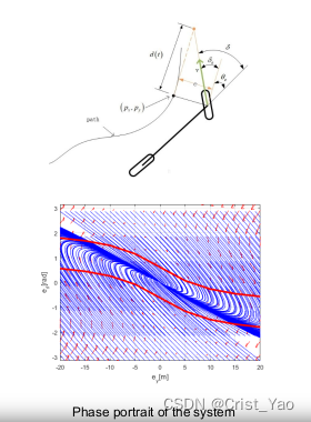
by the above formula $\delta_{_e}=tan^{-1}\frac{ke}{v_{_f}}$

Lateral error distance: $\frac{ke}{v_{_f}}$ ,d(t)=1;

so: $v_{_f}(t)=\sqrt{1+(\frac{ke(t)}{v_{_f}})^{2}}$

$\dot{e}(t)=-v_{_f}(t)sin(\delta_{_e})=-v_{_f}sin(tan^{-1}(\fraction(t)}{v_ {_f}(t)}))=\fraction(t)}{\sqrt{1+(\fraction(t)}{v_{_f}})^{2}}}$

For a very small lateral error, that is, the denominator of the above equation is 1, so $\dot{e}(t)\approx -ke(t)$

K--Natural Index

It can be seen that the natural exponential decay makes the system stable;

Adjustments to Stanley's algorithm

Reverse speed can lead to numerical instability

Add a positive value term to the controller to ensure that the denominator is a positive number;

$\delta(t) = \theta_{_e}(t)+tan^{-1}(\frac{ke(t)}{v_{_f}(t)+k_{_s}})$

Among them $k_{_s}$ > 0 ensures that the denominator has a value greater than 0 to ensure stability;

You can also add a feedforward term to the original Stanley formula:

$\delta = P_{_D}[\theta_{_e}] + arctan(\frac{ke}{ks+k_{_f}})+d_{_ff}(k)$

The Stanley method is easier to adjust than Pure Pursuit, but

There are similar pitfalls when tuning.

• Stanley trackers can be over-tuned to specific scenarios in a similar way

Because the only way it can overcome dynamic effects is to have high gain causing instability on other paths.

• Compared to the Pure Pursuit, a finely tuned Stanley tracker doesn’t “cut corners”;

Instead, it's an overshoot turn. This effect can be attributed to the failure to consider follow-up, similar to pure pursuit;

v has an impact on the front wheel turning angle;

stanley trajectory tracking algorithm

Guess you like