本系列博文为深度学习/计算机视觉论文笔记，转载请注明出处

标题：Unpaired Image-to-Image Translation Using Cycle-Consistent Adversarial Networks

链接：[1703.10593] Unpaired Image-to-Image Translation using Cycle-Consistent Adversarial Networks (arxiv.org)

摘要

图像到图像的转换是一类涉及视觉和图形问题的任务，其目标是通过一组配准的图像对训练集来学习将输入图像映射到输出图像。然而，在许多任务中，很难获得配对的训练数据。我们提出了一种方法，用于在没有配对样本的情况下学习从源领域 $X$ 到目标领域 $Y$ 的图像转换。我们的目标是学习一个映射 $\rightarrow Y$ ，使得从 $G (X)$ 产生的图像分布在使用对抗性损失时与领域 Y 的分布不可区分。由于这种映射存在很大的不确定性，因此我们引入了一个逆映射 $\rightarrow X$ , and introduce a cycle consistency loss to enforce that $\approx X$ (and vice versa). We demonstrate qualitative results without paired training data on multiple tasks, including style transfer, object deformation, season transfer, photo enhancement, and more. The superiority of our method is demonstrated by quantitative comparison with several previous methods.

1 Introduction

What did Claude Monet see when he set up his easel near the Château de Argenteuil-sur-Seine on a beautiful spring day in 1873? Had color photography been invented, it might have been possible to record clear blue skies and glassy river waters reflected in them. Monet, however, expresses his impression of the same scene through soft brushwork and bright color palette.

What would it have been like if Monet had come to the small port of Cassis on a cool summer evening? Looking through a series of Monet's paintings, we can imagine how he would have depicted the scene: perhaps using muted tones, rough paint smears and a flatter dynamic range.

Although we never see Monet's paintings side by side with photographs of the scenes he painted, we know of collections of Monet's paintings and collections of landscape photographs. We can reason about the stylistic differences between the two sets and thus imagine what it would be like to "transform" a scene from one set to the other.

In this paper, we propose a method that can achieve a similar effect: capturing special features of one set of images and figuring out how to transfer those features to another set of images, all without any paired training examples. case.

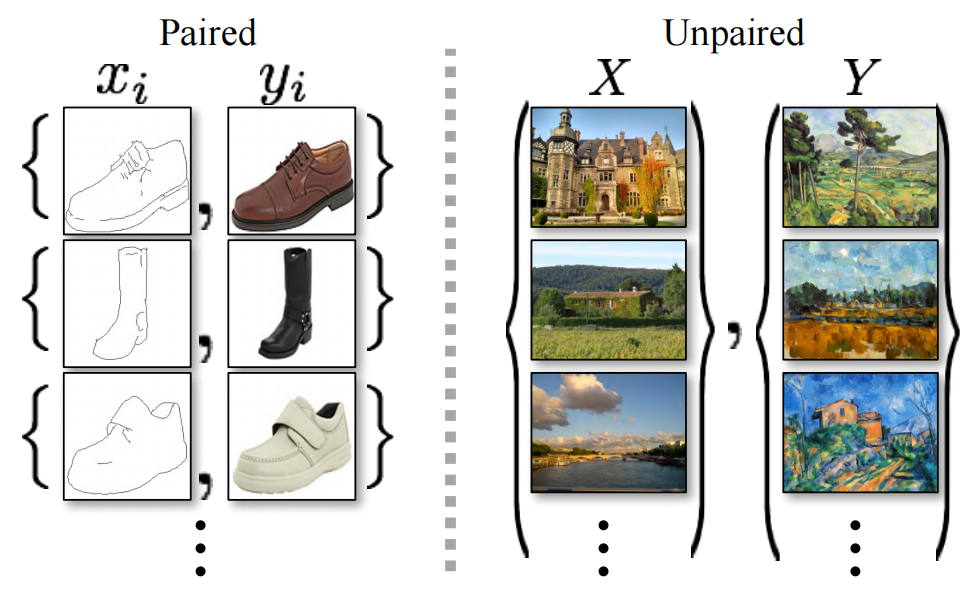
The problem can be more broadly described as image-to-image translation, converting a given scene representation, $x$ , converted to another representation, $y$ , for example, from grayscale to color, from image to semantic label, from edge map to photo. Over the years, research in the fields of computer vision, image processing, computational photography, and graphics has yielded powerful translation systems in supervised settings, where example image pairs { xi , yi } i = 1 N \{x_i, $y_i \}_{i=1}^N$ (Fig. 2, left), for example [11, 19, 22, 23, 28, 33, 45, 56, 58, 62]. However, obtaining paired training data can be difficult and expensive. For example, for tasks like semantic segmentation, only a few datasets exist (e.g. [4]), and they are relatively small. Obtaining input-output pairs is even more difficult for graphics tasks such as artistic stylization, because the required output is very complex and often requires artistic creation. For many tasks, like object deformation (e.g. zebra ↔ horse, top in Figure 1), the desired output is not even well defined.

Figure 1: Given any two unordered collections of images X and Y, our algorithm learns to automatically "translate" between these two sets of images, turning one set of images into the other and vice versa : (left) Monet painting and landscape photos from Flickr; (middle) zebras and horses from ImageNet; (right) summer and winter Yosemite photos from Flickr. Example application (bottom): Using a collection of paintings by famous artists, our method learns to render natural photos into corresponding artistic styles.

Figure 2: The paired training data (left side) consists of training examples { $x_i, y_i$ $x_{i}, y_{i}$ }, among which $x_i$ give $y_i$ There is a corresponding relationship between them [22]. Instead, we consider the unpaired training data (on the right), given by the source set { $x_i$ $x_{i}$ }（ $x_i \in X$ ) and target set { $y_j$ $y_{j}$ }（ $y_j \in Y$ ), but does not provide which $x_i$ with which $y_j$ corresponding information.

We therefore seek an algorithm that can learn to transition between domains without paired input-output examples (Fig. 2, right). We assume some fundamental relationship between domains—for example, they are two different representations of the same underlying scene—and try to learn that relationship. Although we lack supervision in the form of paired examples, we can exploit supervision at the ensemble level: we Given a set of images in $X$ Given another set of images in $Y.$ We can train a mapping $\rightarrow Y$ , such that the output $y^{'} = G (x)$ ，其中 $\in X$ , trained by an adversarial classifier to match domainImage y in $Y$ $\in Y$ is indistinguishable. In theory, this goal can lead to a question about $y^{'}$ , which is consistent with the empirical distribution $p_{\text{data}}(y)$ matches (in general, this requires $G$ is random) [16]. Thus, the optimal $G$ will field $X$ is converted to $The distribution of Y$ is exactly the same as the domain $Y^{'}$ 。

However, such conversion does not guarantee that an individual input $x$ and output $y$ are matched pairwise in meaningful ways - there are infinitely many mappings $G$ , would result in the same $y^{'}$ distribution. Furthermore, in practice, we find it difficult to optimize adversarial objectives individually: standard procedures often lead to the well-known mode collapse problem, where all input images map to the same output image, and optimization fails to make progress.

These problems require us to add more structure to the target. Therefore, we exploit the property that translations should be "cyclically consistent", i.e. if we translate a sentence from English to French and then from French back to English, we should return to the original sentence. Mathematically, if we have a translator $\rightarrow Y$ and another translator $\rightarrow X$ , then $G$ and $F$ should be inverse maps of each other, and both maps should be bijective. by simultaneously training $G$ and $F$ , and adding a cycle consistency loss [64], encourages $\approx x$ 和 $\approx y$ . Comparing this loss with the field $X$ 和 $The combination of adversarial losses on Y$ yields our full objective for unpaired image-to-image translation.

We apply our method to a wide range of applications, including ensemble style transfer, object morphing, season transfer, and photo enhancement. We also compare with previous methods that rely either on manually defined style and content decomposition or on shared embedding functions, and show that our method outperforms these baselines. We provide PyTorch and Torch implementations. Check out more results on our website.

2. Related work

Generative Adversarial Networks (GANs) [16, 63] have achieved impressive results in image generation [6, 39], image editing [66] and representation learning [39, 43, 37]. Recent approaches apply the same ideas to conditional image generation applications such as text-to-image [41], image inpainting [38] and future prediction [36], as well as other domains such as video [54] and 3D data [57]. Key to the success of GANs is the idea of an adversarial loss that forces generated images to be indistinguishable from real photos in principle. This loss is especially effective for image generation tasks, as this is what many goals in computer graphics are optimized for. We employ an adversarial loss to learn a mapping such that the transformed images are indistinguishable from those in the target domain.

Image-to-image translation The idea of image-to-image translation goes back at least to the “image analogy” of Hertzmann et al. [19], who used a non-parametric texture model [10] on a single input-output training image pair. More recent approaches use input-output example datasets to learn parameterized translation functions using CNNs (e.g. [33]). Our approach builds on the "pix2pix" framework of Isola et al. [22], which uses conditional generative adversarial networks [16] to learn a mapping from input to output images. Similar ideas have been applied to various tasks such as generating photos from sketches [44] or generating photos from attributes and semantic layouts [25]. However, unlike the previous work mentioned above, we learn the mapping without paired training examples.

Pairless image-to-image translation Other methods also deal with the pairless setting, where the goal is to relate two data domains: X and Y. Rosales et al. [42] propose a Bayesian framework that includes block-based Markov random field priors computed on source images and likelihood terms obtained from multiple style images. More recently, CoGAN [32] and Cross-Modal Scene Network [1] use a weight sharing strategy to learn common representations across domains. Concurrent with our approach, Liu et al. [31] added a combination of variational autoencoders [27] and generative adversarial networks [16] to the above framework. Parallel lines of work [46, 49, 2] encourage input and output to be shared on specific "content" features, even though they may differ in "style". These methods also use adversarial networks, with additional terms forcing the output to approximate the input in a predefined metric space, such as class label space [2], image pixel space [46] and image feature space [49].

Unlike the aforementioned approaches, our formulation does not rely on task-specific, predefined similarity functions between inputs and outputs, nor does it assume that inputs and outputs must lie in the same low-dimensional embedding space. This makes our method a general solution to many vision and graphics tasks. We directly compare with several previous and contemporaneous methods in Section 5.1.

Loop Consistency Using transitivity as a way to normalize structured data has a long history. Enforcing simple forward-backward consistency has been a standard trick for decades in visual tracking [24, 48]. In the linguistic domain, validating and improving translations through “back-translation and reconciliation” is a technique used by human translators [3] (including, humorously, by Mark Twain [51]) as well as machines [17]. More recently, higher order cycle consistency has been used in terms of motion structure [61], 3D shape matching [21], co-segmentation [55], dense semantic alignment [65, 64] and depth estimation [14]. Among them, Zhou et al. [64] and Godard et al. [14] are the closest to our work, as they use cycle consistency loss as a way to train CNNs with transitive supervision. In this work, we introduce a similar loss so that $G$ and $F$ are consistent with each other. Concurrent with our work, in these same conferences, Yi et al. [59] independently used a similar objective for pair-free image-to-image translation, inspired by bidirectional learning in machine translation.

Neural Style Transfer Neural Style Transfer [13, 23, 52, 12] is another approach to image-to-image translation by combining the content of one image with the style (usually painterly) of another, based on matching Gram matrix statistics for pretrained deep features. In contrast, our main focus is on learning a mapping between two image collections rather than between two specific images, trying to capture the correspondence between higher-level appearance structures. Therefore, our method can be applied to other tasks, such as painting→photo, object deformation, etc., where single-shot transformation methods cannot perform well. We compare these two methods in Section 5.2.

3. Formulation

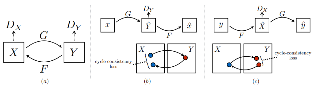
Our goal is to give training samples ${x_i\}_{i=1}^N$ ，其中 $x_i \in X$ ，和 ${y_j\}_{j=1}^M$ ，其中 $y_j \in Y$ ¹, study two domains $X$ 和The mapping function between $Y.$ We denote the data distribution as $\sim p_{\text{data}}(x)$ 和 $\sim p_{\text{data}}(y)$ . As shown in Figure 3(a), our model includes two maps $\rightarrow Y$ 和 $\rightarrow X$ . Furthermore, we introduce two adversarial discriminators $D_X$ 和 $D_Y$ , where $D_X$ Designed to distinguish images ${x\}$ and the translated image ${F(y)\}$ , same place, $D_Y$ Designed to differentiate between ${y\}$ and ${G(x)\}$ . Our objective contains two types of terms: the adversarial loss [16] is used to match the generated image distribution with the data distribution in the target domain; the cycle consistency loss is used to prevent the learned mapping $G$ and $F$ contradicts each other.

Figure 3: (a) Our model contains two mapping functions $\rightarrow Y$ 和 $\rightarrow X$ , and the associated adversarial discriminator $D_Y$ and $D_X$ 。 $D_Y$ Prompt $G$ will $Convert X$ to $Output in Y$ indistinguishable result, for $D_X$ and So is $F.$ To further regularize these mappings, we introduce two cycle consistency losses, capturing the intuition that if we translate from one domain to another and back again, we should be back to the starting point: (b) forward cycle consistency Sex loss: $\rightarrow G(x) \rightarrow F(G(x)) \approx x$ , and © reverse cycle consistency loss: $\rightarrow F(y) \rightarrow G(F(y)) \approx y$ 。

3.1. Adversarial Loss

We apply an adversarial loss [16] to both mapping functions. For the mapping function $\rightarrow Y$ and its discriminator $D_Y$ , we express the objective as:

$L_{\text{GAN}}(G, D_Y, X, Y) = E_{y \sim p_{\text{data}}(y)}[\log D_Y(y)] + E_{x \sim p_{\text{data}}(x)}[\log(1 - D_Y(G(x)))] \tag{1}$

where $G$ tries to generate a field similar toImage G of $Y$ $G (x)$ ，而 $D_Y$ Aims to distinguish translation samples $G (x)$ and the real sample $y$ 。 $G$ aims to minimize this objective, while the opponent $D$ then tries to maximize it, ie:

$\min_G \max_{D_Y} L_{\text{GAN}}(G, D_Y, X, Y)$

We also for the mapping function $\rightarrow X$ and its discriminator $D_X$ Introducing a similar adversarial loss:

$\min_F \max_{D_X} L_{\text{GAN}}(F, D_X, Y, X)$

3.2. Cycle Consistency Loss

In theory, adversarial training can learn to map $G$ and $F$ so that its output is in the target field $Y$ and $The distributions in X$ are exactly the same (strictly speaking, this requires that $G$ and $F$ is a random function) [15]. However, with a sufficiently large capacity, the network can map the same set of input images to any randomly permuted image in the target domain, and any learned mapping can steer the output distribution to match the target distribution. Therefore, there is no guarantee that the learned function will be able to convert a single input $x_i$ maps to the desired output $y_i$ . To further reduce the space of possible mapping functions, we believe that the learned mapping functions should be cycle-consistent: as shown in Figure 3(b), for $X$ 's image $x$ , the image transformation loop should be able to convert $x$ brings back the original image, ie $\rightarrow G(x) \rightarrow F(G(x)) \approx x$ . We call this forward cycle consistency. Similarly, as shown in Fig. 3©, for $Y$ 's image $y$ ， $G$ and $F$ should also satisfy reverse cycle consistency: $\rightarrow F(y) \rightarrow G(F(y)) \approx y$ . We use a cycle consistency loss to incentivize this behavior:

$L_{\text{cyc}}(G, F) = E_{x \sim p_{\text{data}}(x)}[\|F(G(x)) - x\|_1] + E_{y \sim p_{\text{data}}(y)}[\|G(F(y)) - y\|_1] \tag{2}$

In preliminary experiments, we also tried replacing the L1 norm in this loss by $F (G (x) )$ andAdversarial loss between $x$ $G (F (and))$ 和 $y$ , but no performance improvement is observed.

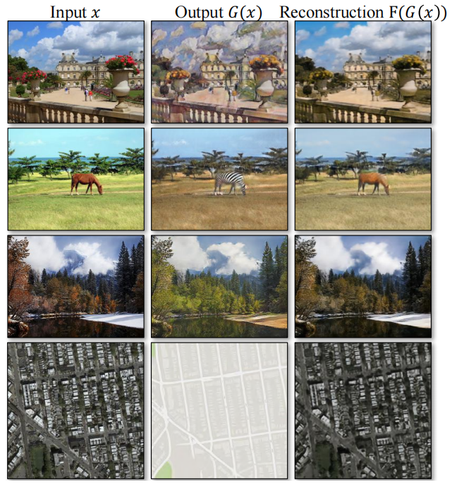
The behavior induced by the cycle consistency loss can be observed in Figure 4: reconstructed image $F (G (x) )$ is finally related to the input image $x$ are very similar.

Figure 4: Input image $x$ , the output image $G (x)$ reconstructed from various experiments $F (G (x))$ . From top to bottom are: photo ↔ Cézanne style, horse ↔ zebra, winter → summer Yosemite, aerial photo ↔ Google Maps.

3.3. Complete goals

Our complete goals are:

$D_X, D_Y) = L_{\text{GAN}}(G, D_Y, X, Y) + L_{\text{GAN}}(F, D_X, Y, X) + \lambda L_{\text{cyc}}(G, F) \tag{3}$

where $\lambda$ controls the relative importance of the two objectives. Our goal is to address:

$G^*, F^* = \arg \min_{G,F} \max_{D_X, D_Y} L(G, F, D_X, D_Y)$

Note that our model can be viewed as training two "autoencoders" [20]: we jointly learn an autoencoder $\circ G: X \rightarrow X$ and another $\circ F: Y \rightarrow Y$ _ However, each of these autoencoders has a special internal structure: they map images to themselves by translating images into translations in another domain. Such a setting can also be viewed as a special case of “adversarial autoencoders” [34] that use an adversarial loss to train the bottleneck layer of the autoencoder to match an arbitrary target distribution. In our case $\rightarrow X$ autoencoder is the domainThe distribution of $Y.$

In Section 5.1.4 we compare our method with L_{\text{GAN}} using only the adversarial loss $L_{\text{GAN}}$ Or just use the cycle consistency loss $L_{\text{cyc}}$ , and empirically show that the two objectives play a key role in achieving high-quality results. We also evaluate in the case of unidirectional recurrent loss, showing that a single recurrent is not sufficient to regularize training for this unconstrained problem.

4. Realize

Network Architecture We adopt the network architecture of Johnson et al. [23], who achieved impressive results in neural style transfer and super-resolution. This network consists of three convolutional layers, several residual blocks [18], two fractional convolutional layers with stride 1/2, and one convolutional layer that maps features to RGB. For 128 × 128 images, we use 6 blocks, and for 256 × 256 and higher resolution training images, we use 9 blocks. Similar to Johnson et al. [23], we use instance normalization [53]. For the discriminator network, we used 70 × 70 PatchGANs [22, 30, 29] whose goal is to classify overlapping 70 × 70 image patches as real or fake. This block-level based discriminator architecture has fewer parameters than full-image discriminators and can handle images of any size in a fully convolutional manner [22].

Training Details We employ two techniques from recent work to stabilize the model training process. First, in LGAN (Equation 1), we replace the negative log-likelihood objective with a least squares loss [35]. This loss is more stable during training, producing higher quality results. In particular, for the GAN loss LGAN(G, D, X, Y), we train G to minimize $E_{x \sim p_{\text{data}}(x)}[(D(G(x)) - 1)^2]$ , train D to minimize $E_{y \ sim p_{\text{data}}(y)}[(D(y) - 1)^2] + E_{x \sim p_{\text{data}}(x)}[D(G(x) )^2]$ 。

Second, to reduce model oscillation [15], we follow the strategy of Shrivastava et al. [46] to update the discriminator using historically generated images instead of images produced by the latest generator. We maintain an image buffer that stores the 50 most recently created images.

$\lambda$ in Equation 3 $λ$ is set to 10. We use the Adam optimizer [26] with a batch size of 1. All networks are trained from scratch with a learning rate of 0.0002. We use the same learning rate for the first 100 epochs, then linearly decrease the learning rate to zero for the next 100 epochs. See the appendix (Section 7) for more details on the dataset, architecture, and training process.

5. Results

We first compare our method with recent unpaired image-to-image translation methods with a paired dataset, where there is real input-output paired data for evaluation. We then investigate the importance of adversarial losses and cycle consistency losses, and compare our full approach with several variants. Finally, we demonstrate the generalizability of our algorithm across a wide range of application domains without paired data. For brevity, we refer to our method as CycleGAN. Code, models and full results for PyTorch and Torch can be found on our website.

5.1 Evaluation

Using the same evaluation dataset and metrics as "pix2pix" [22], we qualitatively and quantitatively compare our method with several baseline methods. Tasks include semantic labeling ↔ photos on the Cityscapes dataset, and maps ↔ aerial photos scraped from Google Maps. We also conduct an ablation study on the full loss function.

5.1.1 Evaluation Indicators

AMT Perception Study For the map↔aerial photo task, we conduct a “real vs fake” perception study on Amazon Mechanical Turk (AMT) to evaluate the authenticity of our output. We followed the perception study protocol of Isola et al. [22] except that we only collected data from 25 participants per algorithm we tested. Participants will see a series of image pairs, one a real photo or map and the other a fake (generated by our algorithm or a baseline method), and then be asked to click on the image they think is real. The first 10 trials of each session are practice sessions, giving participants correct or incorrect responses. The remaining 40 trials were used to assess the rate at which each algorithm fooled participants. Only one algorithm is tested per session, and participants are only allowed to complete one session. The data we report are not directly comparable to those in [22] ^because our benchmark images were lightly processed and we tested with a different population of participants than in [22] (due to run the experiment on a different date and time). Therefore, our data should only be used to compare our current method with a baseline method (running the baseline method under the same conditions), not with [22].

FCN Score While perception studies may be the gold standard for assessing graphical realism, we would also like to have an automatic quantitative measure that does not require human experimentation. To this end, we adopted the "FCN score" from [22] and used it to evaluate the Cityscapes Label→Photo task. The FCN metric evaluates the interpretability of generated photos under an externally pretrained semantic segmentation algorithm (Fully Convolutional Network FCN from [33]). The FCN predicts a label map for the generated photos. This label map can then be compared to the input ground truth labels using standard semantic segmentation metrics described below. The core idea is that if we generate a photo from a "cars on the road" label map, then when applied to the generated photo, the FCN should detect "cars on the road".

Semantic Segmentation Metrics To evaluate performance on the photo→label task, we use standard metrics from the Cityscapes benchmark dataset [4], including per-pixel accuracy, per-class accuracy, and average class intersection-over-union ratio (Class IOU) [4].

5.1.2 Benchmark method

CoGAN [32] This method learns a GAN generator for domain X and a generator for domain Y, where the weights of the first few layers are the same for a shared latent representation. Transformation from X to Y can be achieved by finding a latent representation that can generate image X, and then rendering this latent representation into style Y.

SimGAN [46] is similar to our approach, and Shrivastava et al. [46] use an adversarial loss to train the translation from X to Y. Regularization term $kx - G(x)k_1$ Used to penalize large changes at the pixel level.

Feature Loss + GAN We also tested a variant of SimGAN [46] where the L1 loss is computed on deep image features from a pretrained network (VGG-16 relu4 2 [47]) instead of RGB pixel values computational. Distances are computed in a deep feature space, sometimes referred to as "perceptual loss" [8, 23].

BiGAN/ALI [9, 7] Unconditional GAN [16] learns a generator G: Z → X that maps random noise z to image x. BiGAN [9] and ALI [7] proposed to also learn the inverse mapping function F: X → Z. While they were originally designed to map a latent vector z to an image x, we achieve the same goal of mapping a source image x to a target image y.

pix2pix [22] We also compared our results with pix2pix [22] , which was trained on paired data, to see how close we could be to this "ceiling" without using any paired data. For a fair comparison, we use the same architecture and details as our method, except for CoGAN [32]. CoGAN is based on a generator that generates images from a shared latent representation, which is incompatible with our image-to-image network. We use a publicly available implementation of CoGAN.

5.1.3 Comparison with baseline methods

As shown in Figures 5 and 6, we were unable to obtain convincing results with any baseline method. However, our method can generate translations of similar quality to fully supervised pix2pix.

Figure 5: Different label↔photo mapping methods trained on Cityscapes images. From left to right: input image, BiGAN/ALI [7, 9], CoGAN [32], feature loss + GAN, SimGAN [46], CycleGAN (our method), pix2pix [22] (training on paired data), and real ground truth images.

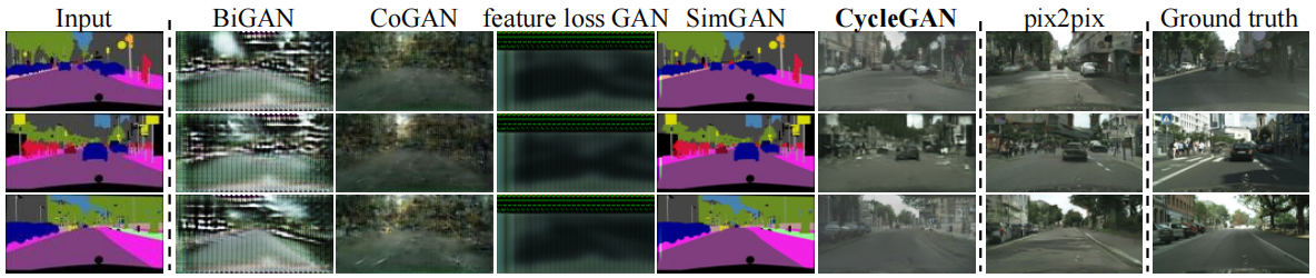
Figure 6: Aerial photo↔map mapping trained on Google Maps by different methods. From left to right: Input, BiGAN/ALI [7, 9], CoGAN [32], Feature Loss + GAN, SimGAN [46], CycleGAN (our method), pix2pix [22] (training on paired data), and Real ground truth.

Table 1 reports the performance related to the AMT perceptual realism task. Here we can see that at 256×256 resolution, our method fooled participants in about a quarter of the trials in both Map→Aerial Photo Direction and Aerial Photo→Map ^Direction3 . All baseline methods almost never fooled the participants.

Table 1: AMT “real vs fake” tests on maps ↔ aerial photos at 256×256 resolution.

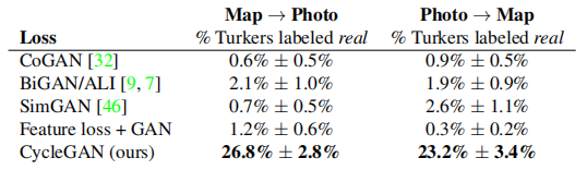
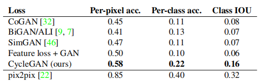
Table 2 evaluates the performance of the label → photo task on the Cityscapes dataset, while Table 3 evaluates the opposite mapping (photo → label). In both cases, our method again outperforms the baseline methods.

Table 2: FCN scores of different methods, evaluated on the Cityscapes dataset for labels→photos.

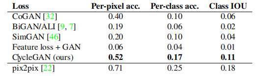
Table 3: Classification performance of different methods on photo → label on the Cityscapes dataset.

5.1.4 Loss function analysis

In Tables 4 and 5 we compare ablation with our full loss. Removing the GAN loss significantly degrades the results, as does removing the cycle consistency loss. Therefore, we conclude that both terms are critical to our results. We also evaluate the recurrent loss of our method with only one direction: GAN + forward recurrent loss $E_{ x \sim p_{\text{data}}(x)}[||F(G(x)) - x||_1]$ , or GAN + reverse loop loss $E_{y \sim p_{\text{data}}(y)} [||G(F(y)) - y||_1]$ (Equation 2), it was found that it tends to cause training instability and trigger mode collapse, especially for the removed mapping directions.

Table 4: Ablation study: FCN scores for different variants of our method, evaluated on the Cityscapes dataset on labels→photos.

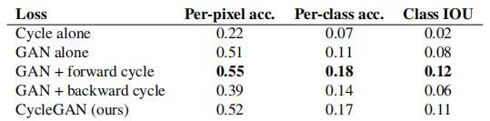
Table 5: Ablation study: classification performance of different loss functions on photo→label, evaluated on the Cityscapes dataset.

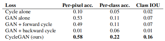
Figure 7 shows some qualitative examples.

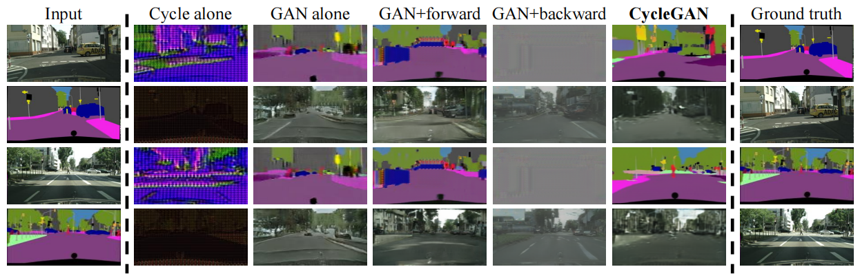
Figure 7: Different variants of label↔photo mapping trained on Cityscapes. From left to right: input, cycle consistency loss only, adversarial loss only, GAN + forward cycle consistency loss ( $\approx x$ ), GAN + reverse cycle consistency loss ( $\approx y$ ), CycleGAN (our full approach), and real ground truth. Both Cycle alone and GAN + reverse fail to generate images similar to the target domain. Both GAN-only and GAN+forward suffer from mode collapse, yielding the same label map independent of the input photo.

5.1.5 Image reconstruction quality

In Fig. 4, we show some reconstructed images $A random sample of F (G (x))$ . We observe that these reconstructed images are often consistent with the original input $x$ is close in both training and testing, even in a domain representing more diverse information, such as maps ↔ aerial photos.

5.1.6 Additional results on paired datasets

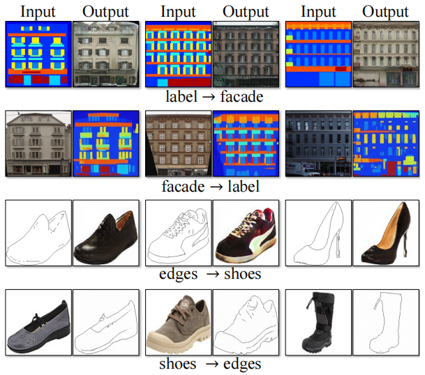
Figure 8 shows some example results on other paired datasets used in “pix2pix” [22], such as building labels↔photos from the CMP Facade Database [40] and fringes ↔ shoes. The image quality of our results is close to that produced by fully supervised pix2pix, while our method learns the mapping without paired supervision.

Figure 8: Example results of CycleGAN on paired datasets used in “pix2pix” [22], such as building labels ↔ photos and edges ↔ shoes.

5.2 Application

We demonstrate our method on several application domains for which paired training data are not available. Please refer to the Appendix (Section 7) for more details on the dataset. We observed that transformations on training data are often more attractive than transformations on test data, and full results for all applications (both training and test data) can be viewed on our project website.

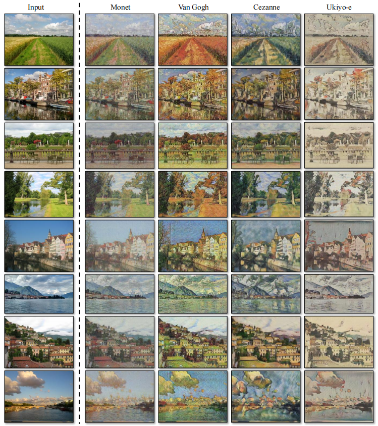
Ensemble Style Transfer (Figures 10 and 11) We train models on landscape photos downloaded from Flickr and WikiArt. Unlike recent work on "neural style transfer" [13], our method learns to imitate the style of an entire collection of artworks, rather than transferring the style of a single selected artwork. So we can learn to generate photos in the style of Van Gogh, not just in the style of Starry Night. The dataset sizes for each artist/style are Cezanne (526), Monet (1073), Van Gogh (400) and Ukiyo-e (563).

Figure 10: Artistic Style Transfer I: We convert the input image to the artistic styles of Monet, Van Gogh, Cezanne, and Ukiyo-e. Please visit our website for more examples.

Figure 11: Artistic Style Transfer II: We convert the input image to the artistic styles of Monet, Van Gogh, Cezanne, and Ukiyo-e. Please visit our website for more examples.

Object Morphing (Fig. 13) The model is trained to transform objects of one ImageNet [5] category into objects of another category (each category contains about 1000 training images). Turmukhambetov et al. [50] proposed a subspace model for transforming one object into another between the same categories, whereas our method focuses on object deformation between two visually similar categories.

Figure 13: Our method applied to multiple translation problems. These images were chosen with relatively successful results - please visit our website for more comprehensive and random results. In the first two rows, we show results on the problem of object translation between horses and zebras, trained on 939 images in the wild horse category and 1177 images in the zebra category of Imagenet [5] . Also check out the Horse→Zebra demo video. The middle two rows show the results of seasonal transformations performed on winter and summer Yosemite photos from Flickr. In the bottom two rows, we trained our method using 996 images of apples and 1020 images of navel oranges from ImageNet.

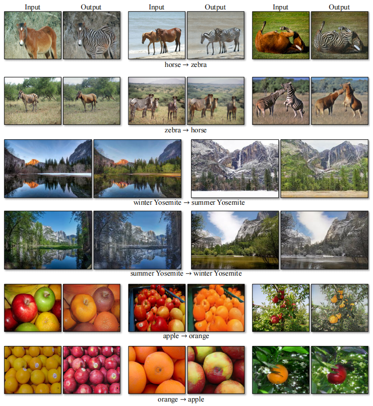
The seasonal transition (Fig. 13) model was trained on 854 winter photos and 1273 summer photos from Yosemite downloaded from Flickr.

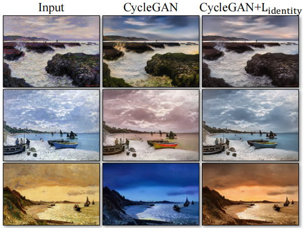
Generating photos from paintings (Fig. 12). For paintings→photos, we find it helpful to introduce an additional loss to encourage the mapping to preserve the color composition between input and output. Specifically, we employ the technique of Taigman et al. [49] to regularize the generator to approximate the identity map when real samples from the target domain are fed to the generator's input: i.e. L identity ( G , F $L_{\text{identity }}(G, F) = E_{y \sim p_{\text{data}}(y)}[||G(y) - y||_1] + E_{x \sim p_{\text{data }}(x)}[||F(x) - x||_1]$ . In the absence of Lidentity, generators G and F are free to change the hue of the input image when it is not necessary. For example, when learning the mapping between paintings from Monet and photos from Flickr, the generator often maps daytime paintings to photos taken at sunset because such a mapping can be equally effective under adversarial losses and cycle consistency losses. Figure 9 shows the effect of this identity mapping loss.

Figure 12: Relatively successful results in translating Monet's paintings into a photographic style. Please visit our website for more examples.

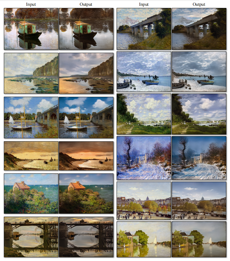
Figure 9: Effect of identity mapping loss on Monet’s painting→photo task. From left to right: Input painting, CycleGAN without identity mapping loss, CycleGAN with identity mapping loss. The identity map loss helps preserve the color of the input painting.

In Figure 12 we show additional results for converting Monet's paintings to photos. This figure and Figure 9 show results on the paintings included in the training set, whereas in all other experiments in the paper we only evaluate and show results on the test set. Because there is no paired data in the training set, it is a very challenging task to come up with a reasonable transformation for the paintings in the training set. Indeed, since Monet is no longer able to create new paintings, generalization to the unseen "test set" paintings is not a pressing problem.

Photo Enhancement (Fig. 14) We show how our method can be used to generate photos with shallow depth of field. We trained the model on photos of flowers downloaded from Flickr. The source domain contains photos of flowers taken by smartphones, usually with a deep depth of field due to the small aperture. The target domain contains photos taken by DSLRs with large apertures. Our model successfully generates photos with shallow depth of field from photos taken by smartphones.

Figure 14: Photo enhancement: Mapped from a set of smartphone snapshots to professional DSLR photos, the system typically learns to generate shallow focus effects. Some of the most successful results in our test set are shown here - the average performance is much worse. Please visit our website for more comprehensive and random examples.

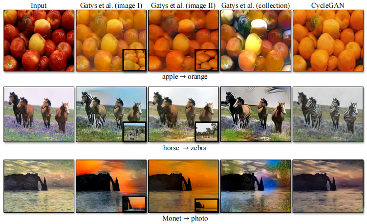
Comparison with Gatys et al. [13] In Fig. 15 we compare our results with neural style transfer [13] on photo stylization. For each row, we first use two typical artworks as style images in [13]. On the other hand, our method can generate photos in the whole collection style. To compare the style of the entire collection with neural style transfer, we compute the average Gram matrix in the target domain and use this matrix to transfer the "average style" of Gatys et al. to our method.

Figure 15: We compare our method with Neural Style Transfer [13] on photo stylization. From left to right: the input image, the result of Gatys et al. [13] using two different representative artworks as the style image, the result of Gatys et al. [13] using the artist's entire collection as the style image, and CycleGAN ( our results).

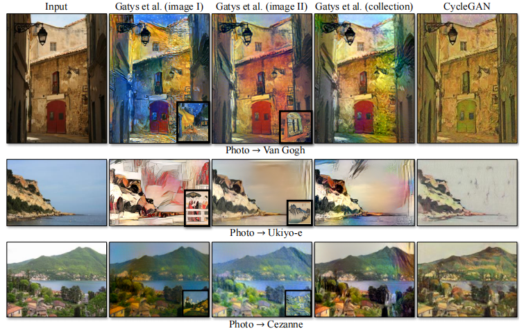
Figure 16 provides a similar comparison for other conversion tasks. We observe that Gatys et al. [13] need to find target-style images that closely match the desired output, but still often fail to produce realistic results, whereas our method successfully generates natural-looking effects similar to the target domain.

Figure 16: We compare our method with neural style transfer [13] on various applications. From top to bottom: apples→oranges, horses→zebras, Monet paintings→photographs. From left to right: the input image, the result of Gatys et al. [13] using two different images as style images, the result of Gatys et al. [13] using all images in the target domain as style images, and CycleGAN (our the result of).

6. Limitations and Discussion

Although our method can achieve convincing results in many cases, the results are not always uniformly positive. Figure 17 shows some typical failure cases. In conversion tasks involving color and texture changes, as in many of the cases reported above, the method usually succeeds. We also tried tasks requiring geometric changes, with little success. For example, in the dog → cat deformation task, the learned transformation becomes the smallest change to the input (Fig. 17). This failure may be due to the fact that our generator architecture is specifically designed for good performance of appearance changes. Handling more kinds and extreme transformations, especially geometric changes, is an important issue for future work.

Figure 17: Typical failure cases of our method. Left: On the dog → cat transformation task, CycleGAN can only make minimal changes to the input. Right: In this horse → zebra example, CycleGAN also fails because our model did not see images of horses while training. See our website for more comprehensive results.

Some failure cases are due to the distribution characteristics of the training dataset. For example, our method confounds in the horse → zebra example (Fig. 17, right) because our model was trained on the wild horse and zebra categories of ImageNet, which does not contain images of people riding horses or zebras. .

We also observe a gap between the results achievable with paired training data and those achieved by our unpaired approach. In some cases, this gap can be very difficult to close, or even impossible: for example, our method sometimes ranks the labels of trees and buildings in the output of the Photo → Label task. Resolving this ambiguity may require some form of weak semantic supervision. Integrating weakly or semi-supervised data may lead to more powerful transformers, but still at a fraction of the annotation cost of fully supervised systems.

Nonetheless, in many cases fully unpaired data are abundantly available and should be exploited. This paper pushes the boundaries of what is possible in this "unsupervised" setting.

Acknowledgments : We thank Aaron Hertzmann, Shiry Ginosar, Deepak Pathak, Bryan Russell, Eli Shechtman, Richard Zhang, and Tinghui Zhou for their many helpful comments on this article. This work was supported in part by NSF SMA-1514512, NSF IIS-1633310, a Google Research Award, Intel Corporation, and hardware donations from NVIDIA. JYZ was supported by a Facebook graduate fellowship, and TP was supported by a Samsung fellowship. Photos used for style transfer were mainly taken in France by AE.

References

Y. Aytar, L. Castrejon, C. Vondrick, H. Pirsiavash, and A. Torralba. Cross-modal scene networks. PAMI,
K. Bousmalis, N. Silberman, D. Dohan, D. Erhan, and D. Krishnan. Unsupervised pixel-level domain adaptation with generative adversarial networks. In CVPR, 2017.
R. W. Brislin. Back-translation for cross-cultural research. Journal of cross-cultural psychology, 1(3):185–216, 1970.
M. Cordts, M. Omran, S. Ramos, T. Rehfeld, M. Enzweiler, R. Benenson, U. Franke, S. Roth, and B. Schiele. The cityscapes dataset for semantic urban scene understanding. In CVPR, 2016.
J. Deng, W. Dong, R. Socher, L.-J. Li, K. Li, and L. Fei-Fei. Imagenet: A large-scale hierarchical image database. In CVPR, 2009.
E. L. Denton, S. Chintala, R. Fergus, et al. Deep generative image models using a Laplacian pyramid of adversarial networks. In NIPS, 2015.
J. Donahue, P. Kr¨ahenb¨uhl, and T. Darrell. Adversarial feature learning. In ICLR, 2017.
A. Dosovitskiy and T. Brox. Generating images with perceptual similarity metrics based on deep networks. In NIPS, 2016.
V. Dumoulin, I. Belghazi, B. Poole, A. Lamb, M. Arjovsky, O. Mastropietro, and A. Courville. Adversarially learned inference. In ICLR, 2017.
A. A. Efros and T. K. Leung. Texture synthesis by non-parametric sampling. In ICCV, 1999.
D. Eigen and R. Fergus. Predicting depth, surface normals and semantic labels with a common multi-scale convolutional architecture. In ICCV, 2015.
L. A. Gatys, M. Bethge, A. Hertzmann, and E. Shechtman. Preserving color in neural artistic style transfer. arXiv preprint arXiv:1606.05897, 2016.
L. A. Gatys, A. S. Ecker, and M. Bethge. Image style transfer using convolutional neural networks. CVPR, 2016.
C. Godard, O. Mac Aodha, and G. J. Brostow. Unsupervised monocular depth estimation with left-right consistency. In CVPR, 2017.
I. Goodfellow. NIPS 2016 tutorial: Generative adversarial networks. arXiv preprint arXiv:1701.00160, 2016.
I. Goodfellow, J. Pouget-Abadie, M. Mirza, B. Xu, D. Warde-Farley, S. Ozair, A. Courville, and Y. Bengio. Generative adversarial nets. In NIPS, 2014.
D. He, Y. Xia, T. Qin, L. Wang, N. Yu, T. Liu, and W.-Y. Ma. Dual learning for machine translation. In NIPS, 2016.
K. He, X. Zhang, S. Ren, and J. Sun. Deep residual learning for image recognition. In CVPR, 2016.
A. Hertzmann, C. E. Jacobs, N. Oliver, B. Curless, and D. H. Salesin. Image analogies. In SIGGRAPH, 2001.
G. E. Hinton and R. R. Salakhutdinov. Reducing the dimensionality of data with neural networks. Science, 313(5786):504–507, 2006.
Q.-X. Huang and L. Guibas. Consistent shape maps via semidefinite programming. In Symposium on Geometry Processing, 2013.
P. Isola, J.-Y. Zhu, T. Zhou, and A. A. Efros. Image-to-image translation with conditional adversarial networks. In CVPR, 2017.
J. Johnson, A. Alahi, and L. Fei-Fei. Perceptual losses for real-time style transfer and super-resolution. In ECCV, 2016.
Z. Kalal, K. Mikolajczyk, and J. Matas. Forward-backward error: Automatic detection of tracking failures. In ICPR, 2010.
L. Karacan, Z. Akata, A. Erdem, and E. Erdem. Learning to generate images of outdoor scenes from attributes and semantic layouts. arXiv preprint arXiv:1612.00215, 2016.
D. Kingma and J. Ba. Adam: A method for stochastic optimization. In ICLR, 2015.
D. P. Kingma and M. Welling. Auto-encoding variational Bayes. ICLR, 2014.
P.-Y. Laffont, Z. Ren, X. Tao, C. Qian, and J. Hays. Transient attributes for high-level understanding and editing of outdoor scenes. ACM TOG, 33(4):149, 2014.
C. Ledig, L. Theis, F. Huszár, J. Caballero, A. Cunningham, A. Acosta, A. Aitken, A. Tejani, J. Totz, Z. Wang, et al. Photo-realistic single image super-resolution using a generative adversarial network. In CVPR, 2017.
C. Li and M. Wand. Precomputed real-time texture synthesis with Markovian generative adversarial networks. ECCV, 2016.
M.-Y. Liu, T. Breuel, and J. Kautz. Unsupervised image-to-image translation networks. In NIPS, 2017.
M.-Y. Liu and O. Tuzel. Coupled generative adversarial networks. In NIPS, 2016.
J. Long, E. Shelhamer, and T. Darrell. Fully convolutional networks for semantic segmentation. In CVPR, 2015.
A. Makhzani, J. Shlens, N. Jaitly, I. Goodfellow, and B. Frey. Adversarial autoencoders. In ICLR, 2016.
X. Mao, Q. Li, H. Xie, R. Y. Lau, Z. Wang, and S. P. Smolley. Least squares generative adversarial networks. In CVPR. IEEE, 2017.
M. Mathieu, C. Couprie, and Y. LeCun. Deep multi-scale video prediction beyond mean square error. In ICLR, 2016.
M. F. Mathieu, J. Zhao, A. Ramesh, P. Sprechmann, and Y. LeCun. Disentangling factors of variation in deep representation using adversarial training. In NIPS, 2016.
D. Pathak, P. Krahenbuhl, J. Donahue, T. Darrell, and A. A. Efros. Context encoders: Feature learning by inpainting. CVPR, 2016.
A. Radford, L. Metz, and S. Chintala. Unsupervised representation learning with deep convolutional generative adversarial networks. In ICLR, 2016.
R. ˇS. Radim Tyleˇcek. Spatial pattern templates for recognition of objects with regular structure. In Proc. GCPR, Saarbrucken, Germany, 2013.
S. Reed, Z. Akata, X. Yan, L. Logeswaran, B. Schiele, and H. Lee. Generative adversarial text to image synthesis. In ICML, 2016.
R. Rosales, K. Achan, and B. J. Frey. Unsupervised image translation. In ICCV, 2003.
T. Salimans, I. Goodfellow, W. Zaremba, V. Cheung, A. Radford, and X. Chen. Improved techniques for training GANs. In NIPS, 2016.
P. Sangkloy, J. Lu, C. Fang, F. Yu, and J. Hays. Scribbler: Controlling deep image synthesis with sketch and color. In CVPR, 2017.
Y. Shih, S. Paris, F. Durand, and W. T. Freeman. Data-driven hallucination of different times of day from a single outdoor photo. ACM TOG, 32(6):200, 2013.
A. Shrivastava, T. Pfister, O. Tuzel, J. Susskind, W. Wang, and R. Webb. Learning from simulated and unsupervised images through adversarial training. In CVPR, 2017.
K. Simonyan and A. Zisserman. Very deep convolutional networks for large-scale image recognition. In ICLR, 2015.
N. Sundaram, T. Brox, and K. Keutzer. Dense point trajectories by GPU-accelerated large displacement optical flow. In ECCV, 2010.
Y. Taigman, A. Polyak, and L. Wolf. Unsupervised cross-domain image generation. In ICLR, 2017.
D. Turmukhambetov, N. D. Campbell, S. J. Prince, and J. Kautz. Modeling object appearance using context-conditioned component analysis. In CVPR, 2015.
M. Twain. The jumping frog: in English, then in French, and then clawed back into a civilized language once more by patient. Unremunerated Toil, 3, 1903.
D. Ulyanov, V. Lebedev, A. Vedaldi, and V. Lempitsky. Texture networks: Feed-forward synthesis of textures and stylized images. In ICML, 2016.
D. Ulyanov, A. Vedaldi, and V. Lempitsky. Instance normalization: The missing ingredient for fast stylization. arXiv preprint arXiv:1607.08022, 2016.
C. Vondrick, H. Pirsiavash, and A. Torralba. Generating videos with scene dynamics. In NIPS, 2016.
F. Wang, Q. Huang, and L. J. Guibas. Image co-segmentation via consistent functional maps. In ICCV, 2013.
X. Wang and A. Gupta. Generative image modeling using style and structure adversarial networks. In ECCV, 2016.
J. Wu, C. Zhang, T. Xue, B. Freeman, and J. Tenenbaum. Learning a probabilistic latent space of object shapes via 3D generative-adversarial modeling. In NIPS, 2016.
S. Xie and Z. Tu. Holistically-nested edge detection. In ICCV, 2015.
Z. Yi, H. Zhang, T. Gong, Tan, and M. Gong. Dual-GAN: Unsupervised dual learning for image-to-image translation. In ICCV, 2017.
A. Yu and K. Grauman. Fine-grained visual comparisons with local learning. In CVPR, 2014.
C. Zach, M. Klopschitz, and M. Pollefeys. Disambiguating visual relations using loop constraints. In CVPR, 2010.
R. Zhang, P. Isola, and A. A. Efros. Colorful image colorization. In ECCV, 2016.
J. Zhao, M. Mathieu, and Y. LeCun. Energy-based generative adversarial network. In ICLR, 2017.
T. Zhou, P. Krahenbuhl, M. Aubry, Q. Huang, and A. A. Efros. Learning dense correspondence via 3D-guided cycle consistency. In CVPR, 2016.
T. Zhou, Y. J. Lee, S. Yu, and A. A. Efros. Flowweb: Joint image set alignment by weaving consistent, pixel-wise correspondences. In CVPR, 2015.
J.-Y. Zhu, P. Kr¨ahenb¨uhl, E. Shechtman, and A. A. Efros. Generative visual manipulation on the natural image manifold. In ECCV, 2016.

7. Appendix

7.1. Training Details

We train the network from scratch with an initial learning rate of 0.0002. In practice, we halve the objective when optimizing the discriminator D to slow down the learning speed of D relative to the speed of G. Maintain the same learning rate for the first 100 epochs, then linearly decay the learning rate to zero for the next 100 epochs. The weights are initialized to a Gaussian distribution N(0, 0.02).

Cityscapes labels ↔ photos : 2975 training images of size 128×128 are obtained from the Cityscapes training set [4]. Tested with Cityscapes validation set.

Maps ↔ Aerial Photos : 1096 training images of size 256×256 were obtained from Google Maps [22]. These images are from New York City and its surrounding areas. Based on the median latitude of the sampling area, the data is split into training and testing sets (buffering regions are added to ensure that no training pixels are included in the testing set).

Building Facade Labels ↔ Photos : 400 training images are obtained from the CMP Facade Database [40].

Edges→Shoes : About 50000 training images are obtained from the UT Zappos50K dataset [60]. The model is trained for 5 epochs.

Horses ↔ Zebras and Apples ↔ Oranges : Images of wild horses, zebras, apples and oranges were downloaded using ImageNet [5]. These images are scaled to 256×256 pixels. The training set sizes for each category are 939 (horse), 1177 (zebra), 996 (apple) and 1020 (orange).

Summer ↔ Winter Yosemite : These images were downloaded using the Flickr API and searching for the tags yosemite and date-taken fields. Black and white photos removed. These images are scaled to 256×256 pixels. The training set size for each category is 1273 (summer) and 854 (winter).

Photo ↔ Artistic Style Transfer : Downloaded artistic images from Wikiart.org. Some sketches or overly explicit artwork were manually culled. Downloaded photos from Flickr using tags landscape and landscapephotography. Black and white photos removed. These images are scaled to 256×256 pixels. The training set sizes for each category are 1074 (Monet), 584 (Cézanne), 401 (Van Gogh), 1433 (Ukiyo-e), and 6853 (photo). Monet's dataset was specifically trimmed to include only landscapes, while Van Gogh's dataset included only his most recognizable artistic styles from later periods.

Monet's painting → photo : To achieve high resolution and save memory, we did a random square crop of the original image. To generate the result, we pass an image with a width of 512 pixels and the correct aspect ratio to the generator network as input. The weight of the identity mapping loss is 0.5λ, where λ is the weight of the cycle consistency loss. We set λ = 10.

Flower Photo Enhancement : Flower images taken with an Apple iPhone 5, 5s, or 6 were downloaded from Flickr by searching for the tag flower. DSLR images with shallow depth of field were also downloaded from Flickr by searching tags flower, dof. The width of these images is scaled to 360 pixels. The weight of the identity mapping loss is 0.5λ. The training set sizes for the smartphone and DSLR datasets are 1813 and 3326, respectively. We set $l = 10$ 。

7.2. Network Architecture

Below is the network architecture of the generator and discriminator. We provide PyTorch and Torch implementations.

Generator Architecture : We adopt the architecture of Johnson et al. [23]. For 128×128 training images, we use 6 residual blocks, and for 256×256 or higher resolution training images, we use 9 residual blocks. The following are the naming conventions we follow in the Johnson et al. GitHub repository.

c7s1-k: 7×7 convolutional-instance normalization-ReLU layer with k filters and stride 1.
dk: 3×3 convolutional-instance normalization-ReLU layer with k filters and stride 2.
Rk: Residual block, consisting of two 3×3 convolutional layers with the same number of filters.
uk: 3×3 fractional strided convolution with k filters and stride 1/2-instance normalization-ReLU layer.

The network using 6 residual blocks is as follows:

c7s1-64,d128,d256,R256,R256,R256,
R256,R256,R256,u128,u64,c7s1-3

The network using 9 residual blocks is as follows:

c7s1-64,d128,d256,R256,R256,R256,
R256,R256,R256,R256,R256,R256,u128
u64,c7s1-3

Discriminator Architecture : For the discriminator network, we use a 70×70 PatchGAN [22]. Ck denotes a 4×4 convolution-instance normalization-LeakyReLU layer with k filters and stride 2. After the last layer, we apply convolution to produce a 1D output. We do not use instance normalization in the first C64 layer. We use Leaky ReLUs with a slope of 0.2. The discriminator architecture is as follows:

C64-C128-C256-C512

Normalization-ReLU layer.