HHU Business Data Mining Final Exam Review

Hohai University Business Intelligence Course Examination Key Points

Special thanks to Liu j for providing the mind map and Lin yt for the modification and supplement

• mind Mapping

Chapter 1 Overview

• information and knowledge

  • information
    • Through certain technologies and methods, the data is integrated and analyzed, and its potential laws and connotations are mined, and the result obtained is information.
    • Information is data with business significance
  • Knowledge
    • When information is used for business decision-making and corresponding business activities are carried out based on the decision-making, the information will be transformed into knowledge. The process of transforming information into knowledge not only needs information, but also needs to combine the experience and ability of decision-makers to solve practical problems.

• System composition of business intelligence (six main components)

  • data source
    • The operational system within the enterprise, that is, the information system that supports the daily operation of each business department
    • External to the business, such as demographic information, competitor information, etc.
  • database
    • Data from various data sources needs to be placed in an environment for analysis after extraction and conversion, so as to manage the data. This is the data warehouse
  • online analytical processing
  • data profiling
  • data mining
  • business performance management

Chapter 2 Business Intelligence Process

2.1 Four parts

• Four sections with questions for each section

• planning

  • In the planning stage, the main goal is to select the business department or business area to implement business intelligence, so as to solve the key business decision-making problems of the enterprise, identify the personnel who use the business intelligence system and the corresponding information needs , and plan the time, cost and resources of the project. use
    • Understand the needs of each business unit or business area, and collect their current urgent needs
    • Question Which business links in the enterprise are costing too much? Which processes are taking too long? In which links the quality of decision-making is not high

• demand analysis

  • Identify requirements considering importance and ease of implementation
  • In terms of importance, it can be measured from three aspects
    • Measuring the Actionability of Information Provided by BI
    • Measuring the return that implementing BI may bring to the business
    • Measuring how implementing BI can help businesses
  • Ease of achieving short-term goals
    • The scope of business intelligence implementation needs to be involved
    • Measuring Data Availability

• design

  • If you want to create a data warehouse, then carry out the model design of the data warehouse, and the multidimensional data model is commonly used . The data mart can extract data from the data warehouse for construction
  • It is also possible to design and implement a data mart directly for a business department without building a data warehouse.
  • If you want to implement OLAP to solve problems, you need to design the aggregation operation type of multidimensional analysis.
  • If you want to use data mining technology, you need to choose a specific algorithm

• accomplish

  • In the implementation stage, select ETL tools to extract source data, build data warehouses and (or) data marts
  • For the data in the data warehouse or data mart, select and apply corresponding query or analysis tools, including enhanced query, reporting tools, online analysis and processing tools, data mining systems, and enterprise performance management tools, etc.
  • Before the specific application of the system, it is necessary to complete the data loading and application testing of the system, and design the access control and security management methods of the system .

2.2 Data warehouse and database

• Relationships represent the majority of data warehouses in two areas

  • The data comes from the database of the business system
  • At present, most data warehouses are managed by database systems.

• Differences: The purpose of construction, the data to be managed, and the management methods are all different

  • The database is mainly used to realize the daily business operation of the enterprise and improve the efficiency of business operation; the construction of the data warehouse is mainly used to integrate data from multiple data sources, and these data are finally used for analysis
  • The database usually only contains the current data, the data storage avoids redundancy as much as possible , and the data organization is implemented according to the data involved in the business process, which is driven by the application. The data in the data warehouse is organized according to the theme, and all the data of a certain theme are integrated together, and there is redundancy in the data .

• Differences: The purpose of construction, the data to be managed, and the management methods are all different

  • The data in the database needs to be updated frequently such as insertion, deletion, modification, etc., and a complex concurrency control mechanism is required to ensure the isolation of transaction operation.
  • The data in the data warehouse is mainly used for analytical processing, except for the initial import and batch data cleanup operations, the data rarely requires update operations
  • The timeliness of the data update operation in the database is very strong , and the throughput rate of the transaction is a very important indicator. However, the data volume of the data warehouse is very large, and the analysis usually involves a large amount of data, and the timeliness is not the most critical. Data quality in a data warehouse is critical , and incorrect data will lead to erroneous analysis results.

2.3 Online Analytical Processing and Online Transaction Processing

Online transaction processing (OLTP) is the main function of the database management system and is used to complete the daily business operations of various departments within the enterprise.

Online analytical processing (OLAP) is the main application of the data warehouse system, providing multi-dimensional analysis of data to support the decision-making process

Chapter Three Correlation Analysis

3.1 Frequent patterns and association rules

1. The concept of frequent patterns

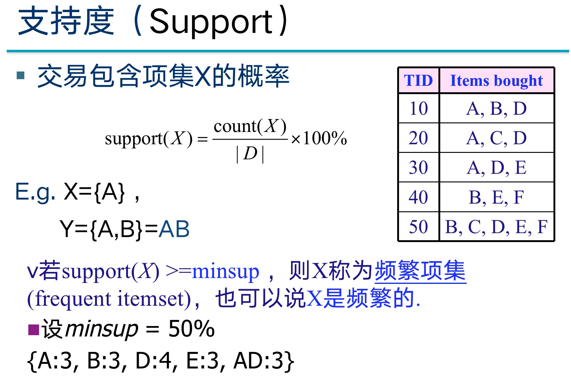
The pattern (which can be a subsequence, substructure, subset, etc.) that often appears in the data set (the frequency of occurrence is not less than minsup, minsup is artificially set, such as 50%) can be applied to sales analysis, web logs Analysis, DNA sequence analysis.

2. The concept of association rules

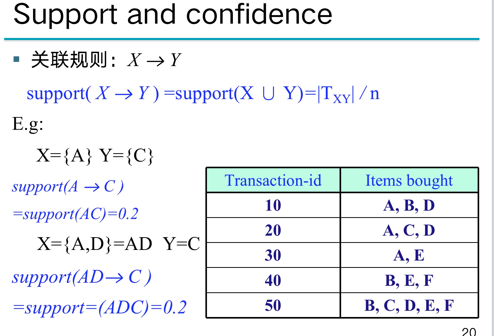
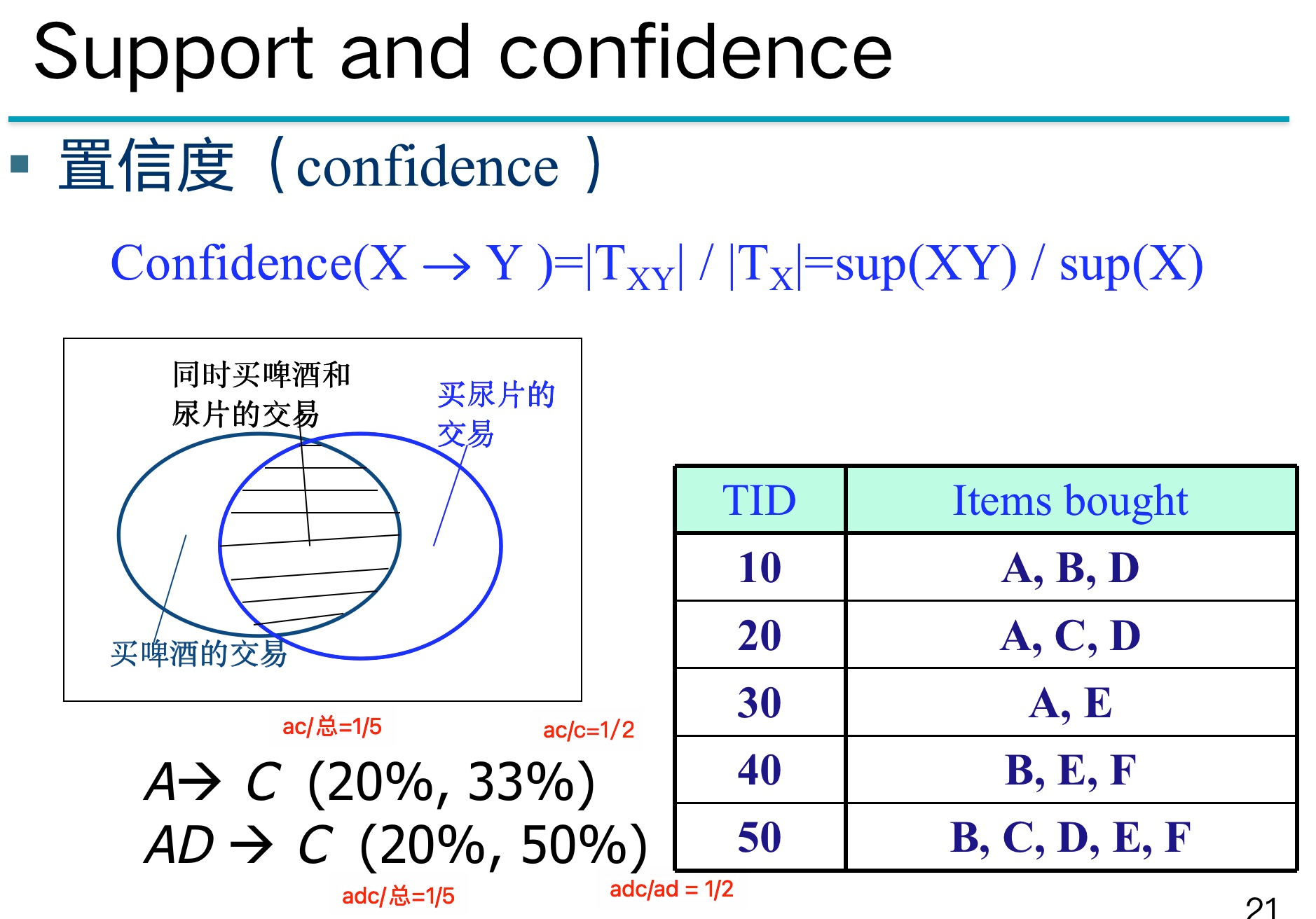
When X appears, Y also appears. X->Y usually has two data, one is the frequency that XY occurs together, and the other is the conditional probability of Y occurring when X occurs.

Link 1: Data Mining Essay (1) Frequent Pattern Mining and Association Rules Mining and Apriori Algorithm (Python Implementation)

Link 2: Frequent Patterns and Association Rules

TIME	transaction
T1	eggs, toothpaste, steak, milk, bread
T2	eggs, flaxseed, olive oil, milk, bread
T3	eggs, puffs, cream, milk, bread
T4	Eggs, Cake Flour, Powdered Sugar, Butter, Milk

For example, our egg milk $A={egg,milk} $,$ bread B={bread} $.

So

$support(A\Rightarrow B)=P(A\cup B)=\frac{3}{4}=0.75$

$D\text{'}$ s transaction contains{eggs, milk, bread} \{eggs, milk, bread\} The entries for$\{$$eggs,\; milk,\; bread$$\}$$T1,T2,T3$ are three in total, so the molecule is 3

$confidence(A\Rightarrow B)=\frac{P(A\cup B)}{P(A)}=\frac{3}{4}=0.75$

A appears in T1~T4, so the denominator is 4, and the numerator is the same as above

Obviously, for the calculated value, we need to set an artificial threshold to determine whether A and B are an association rule. Suppose we set two thresholds $s$ and$c$ . Then if$support(A\Rightarrow B)\ge s\wedge confidence(A\Rightarrow B)\ge c$ , we say$A\Rightarrow B$ is an association rule. Its actual meaning is to buy$eggs,Milk$ is likely to buy$bread$ .

This is the simplest method of association rule mining, so we can summarize the steps of association rule mining in two steps:

1. Find all possible frequent itemsets . A frequent itemset is defined as an itemset whose occurrence frequency of support in the transaction set is greater than the set threshold min_sup.
2. Generate strong association rules in the found frequent itemsets. The frequent itemset pairs conforming to the strong association rules need to meet the requirement that their support and confidence are both greater than the preset thresholds.

• for example

  • 
  • 

• There is a small mistake here, con(A->C) should be ac/a=1/3

3.2 Correlation measure

Generally, we use three indicators to measure an association rule, these three indicators are: support, confidence and promotion.

Support (support): Indicates the proportion of transactions containing both A and B to all transactions. If P(A) is used to represent the proportion of using A transaction, then Support=P(A&B)

Confidence (credibility): Indicates the proportion of transactions containing A and transactions containing B, that is, the proportion of transactions containing both A and B to transactions containing A. Formula expression: Confidence=P(A&B)/P(A)

Lift (lift): Indicates the ratio of "proportion of transactions containing A that also contain transactions B" to "proportion of transactions containing B". Formula expression: Lift=(P(A&B)/P(A))/P(B)=P(A&B)/P(A)/P(B).

The lift reflects the correlation between A and B in the association rules. The lift > 1 and higher indicates a higher positive correlation, the lift < 1 and lower indicates a higher negative correlation, and the lift = 1 indicates no correlation sex.

for example:

10,000 supermarket orders (10,000 transactions), of which 6,000 are for the purchase of Sanyuan milk (transaction A), 7,500 are for the purchase of Yili milk (transaction B), and 4,000 include both.

Then through the calculation method of the above support, we can calculate:

**The support degree of Sanyuan Milk (A transaction) and Yili Milk (B transaction) is: **P(A&B)=4000/10000=0.4.

**The confidence degree of Sanyuan Milk (A transaction) to Yili Milk (B transaction) is: **The proportion of transactions that include A in the transactions that also include B accounts for the transaction that includes A. 4000/6000=0.67, it means that after buying Sanyuan milk, 0.67 users will buy Yili milk.

**The confidence level of Yili milk (transaction B) on ternary milk (transaction A) is: **The proportion of transactions that also contain A among the transactions that include B accounts for the proportion of transactions that include B. 4000/7500=0.53, it means that after buying Sanyuan milk, 0.53 users will buy Yili milk.

Above we can see that transaction A has a confidence level of 0.67 for transaction B, which seems to be quite high, but it is actually misleading. Why do you say that?

Because without any conditions, the occurrence ratio of transaction B is 0.75, while the ratio of transaction A and transaction B at the same time is 0.67, that is to say, if the condition of transaction A is set, the ratio of transaction B will decrease instead . This shows that A transaction and B transaction are exclusive.

The following is the concept of lift.

We take the ratio of 0.67/0.75 as the promotion degree, that is, P(B|A)/P(B), which is called the promotion degree of A condition to B transaction, that is, with A as the premise, what is the probability of B appearing If the promotion degree = 1, it means that A and B are not related in any way. If <1, it means that A transaction and B transaction are exclusive. > 1, we think that A and B are related, but in specific applications , we think that the lift degree > 3 can be regarded as an association worthy of recognition.

lift

In fact, if sup is used to represent the frequency of occurrence of a certain item (note that it is not frequency, sup in the above figure is frequency), n represents the total number of items, for example, here is n, then lift ( A ⇒ B ) = sup ( $lift(A\Rightarrow B)=\frac{sup\left(AB\right)\ast }{sup(A)sup(B)}$

cosine

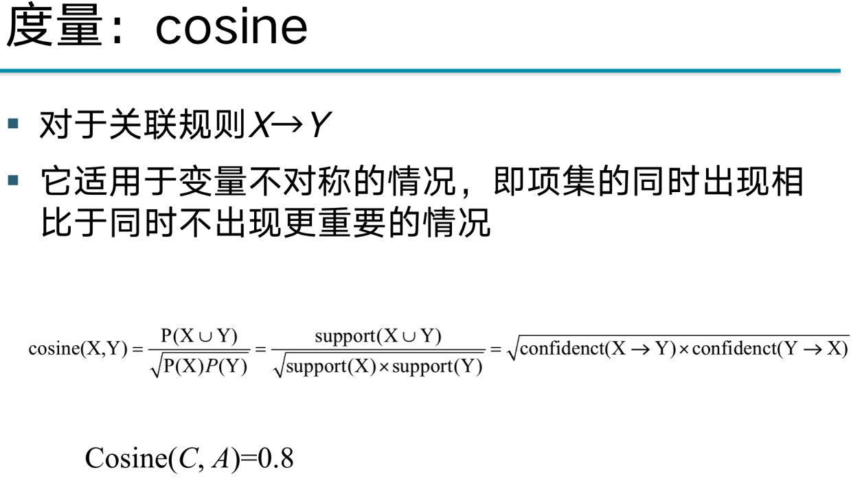
The root sign is opened below, so there is no need to calculate the n. directly $\frac{sup(AB}{\sqrt{sup(A)sup(B)}}$, remind me again that the sup here is the number of occurrences

Chapter IV Classification

• Classification: the process of summarizing the characteristics of objects of existing categories and then predicting the categories of objects of unknown categories
• classifier
• training dataset
  • Class label attribute, each value is called a class (class label), which is the label y
  • Attribute, used to describe a certain characteristic or property of an object, is the feature x
• testing dataset

4.1 Decision tree

• build process

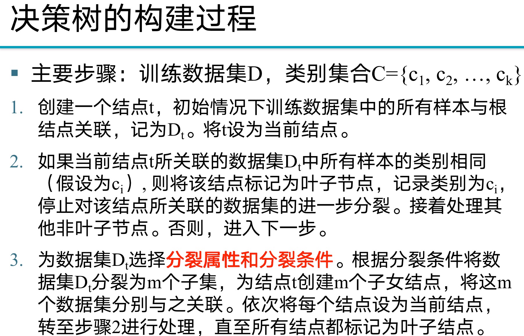
• Selection of Splitting Attributes and Splitting Conditions
  • The selection of splitting attributes usually utilizes a measure of class purity as a criterion
  • Two types of information entropy and gini index

4.1.1 The concept of information entropy

• The size of information entropy can be considered as the size of the information needed to continue to figure out things. First, there is a concept, which we will review later

4.1.2 Calculate the information entropy of the target variable

• The full text is represented by this example

The weather predicts whether to play basketball. Suppose we have the following data:

Weather	Play Basketball
Sunny	Yes
Overcast	Yes
Rainy	Yes
Sunny	Yes
Sunny	No
Overcast	Yes
Rainy	No
Rainy	No
Sunny	Yes

where "Weather" is the feature and "Play Basketball" is the target variable. We want to calculate the information entropy when splitting the data with "Weather" as the node.

First, we want to calculate the entropy of the target variable "Play Basketball" with the formula:

$H(X)=-\sum P(x){\log }_{2}P\left(x\right)$

In this example, we have 6 "Yes" and 3 "No", so the entropy of Play Basketball is:

$H(PlayBasketball)=-[(6/9)\ast log2(6/9)+(3/9)\ast log2(3/9)]$

We can calculate that $ H(Play Basketball) ≈ 0.918$.

Supplement: Information entropy is a measure of the degree of chaos or uncertainty of a data set. When all the data in the data set belong to the same category, the uncertainty is the smallest, and the information entropy at this time is 0.

• If all rows belong to the same category, for example, all are "Yes", then we can get according to the formula of information entropy:

$Entropy=-\sum P(x){\log }_{2}P\left(x\right)=-[1\ast log2(1)+0]=0$

where $P\left(x\right)$ is the probability of a particular class.

• When the two categories are evenly distributed, for example, "Yes" and "No" each account for half, that is, the probability is 0.5, then the uncertainty is the largest, and the information entropy at this time is 1.

If the two categories are evenly distributed, we can get according to the formula of information entropy:

$Entropy=-\sum P(x){\log }_{2}P\left(x\right)=-[0.5\ast log2(0.5)+0.5\ast log2(0.5)]=1$

• So, when building a decision tree, our goal is to find a way to divide the data into as pure (ie low entropy) subsets as possible.

4.1.3 Calculate conditional entropy

After calculating the information entropy of the target variable above, we need to calculate the conditional entropy of each feature. The formula of the conditional entropy is:

$H(Y|X)=\sum P(x)H(Y|x)$

where $P\left(x\right)$ is the probability distribution of feature X,$H(Y|x)$ is the entropy of Y given X.

Count the data of the example

Weather	Play Basketball = Yes	Play Basketball = No
Sunny	3	1
Overcast	2	0
Rainy	1	2

For example, if we split the data with "Weather" as the node

• The conditional entropy of "Sunny" is:

$H(PlayBasketball|Weather=Sunny)=-[(2/3)\ast log2(2/3)+(1/3)\ast log2(1/3)]\approx 0.811$

• For "Overcast" weather:

$H(PlayBasketball|Weather=Overcast)=-[1\ast log2(1)+0]=0$

• For "Rainy" weather:

$H(PlayBasketball|Weather=Rainy)=-[(1/3)\ast log2(1/3)+(2/3)\ast log2(2/3)]\approx 0.918$

• Then, we need to calculate the conditional entropy when splitting the data with "Weather" as the node. This requires summing the conditional entropy for each weather combined with the probability of the weather (in this case the probability of Weather=Sunny, Overcast, Rainy):

$H(PlayBasketball|Weather)=P(Sunny)\ast H(PlayBasketball|Weather=Sunny)+P(Overcast)\ast H(PlayBasketball|Weather=Overcast)+P(Rainy)\ast H(PlayBasketball|Weather=Rainy)=(4/9)\ast 0.811+(2/9)\ast 0+(3/9)\ast 0.918\approx 0.764$

4.1.4 Information Gain

Finally, we can subtract the conditional entropy from the entropy of the target variable to obtain the information gain when splitting the data with "Weather" as the node. The larger the information gain, the better the data split with this feature as the node.

$Gain(Weather)=H(PlayBasketball)-H(PlayBasketball|Weather)=0.918-0.764=0.154$

This result shows that using "Weather" as the node for division can bring an information gain of 0.154, which helps us decide whether to choose "Weather" as the node for division.

4.1.5 Supplement

• From knowing the question, first of all, we need to understand what information entropy is

First of all, two kinds of information are distinguished: the amount of information needed to continue to figure out the thing VS the amount of information provided by previously known information. Information entropy changes in the same direction as the amount of information needed to continue to figure out the thing , and information entropy changes in the opposite direction to the amount of information provided by previously known information.

The greater the information entropy, the greater the uncertainty of things, so the greater the amount of information needed to continue to figure out the thing, this means that the previously known information or the previously known data provides less information;

The smaller the information entropy, the smaller the uncertainty of things, so the amount of information needed to continue to figure out the thing is smaller, which means that the amount of information provided by previously known information or previously known data is greater.

• The greater the information entropy of a random variable, the greater the amount of information its value (content) can give you, and the smaller the amount of information you have before knowing this value

4.1.6 Types of attributes and splitting conditions

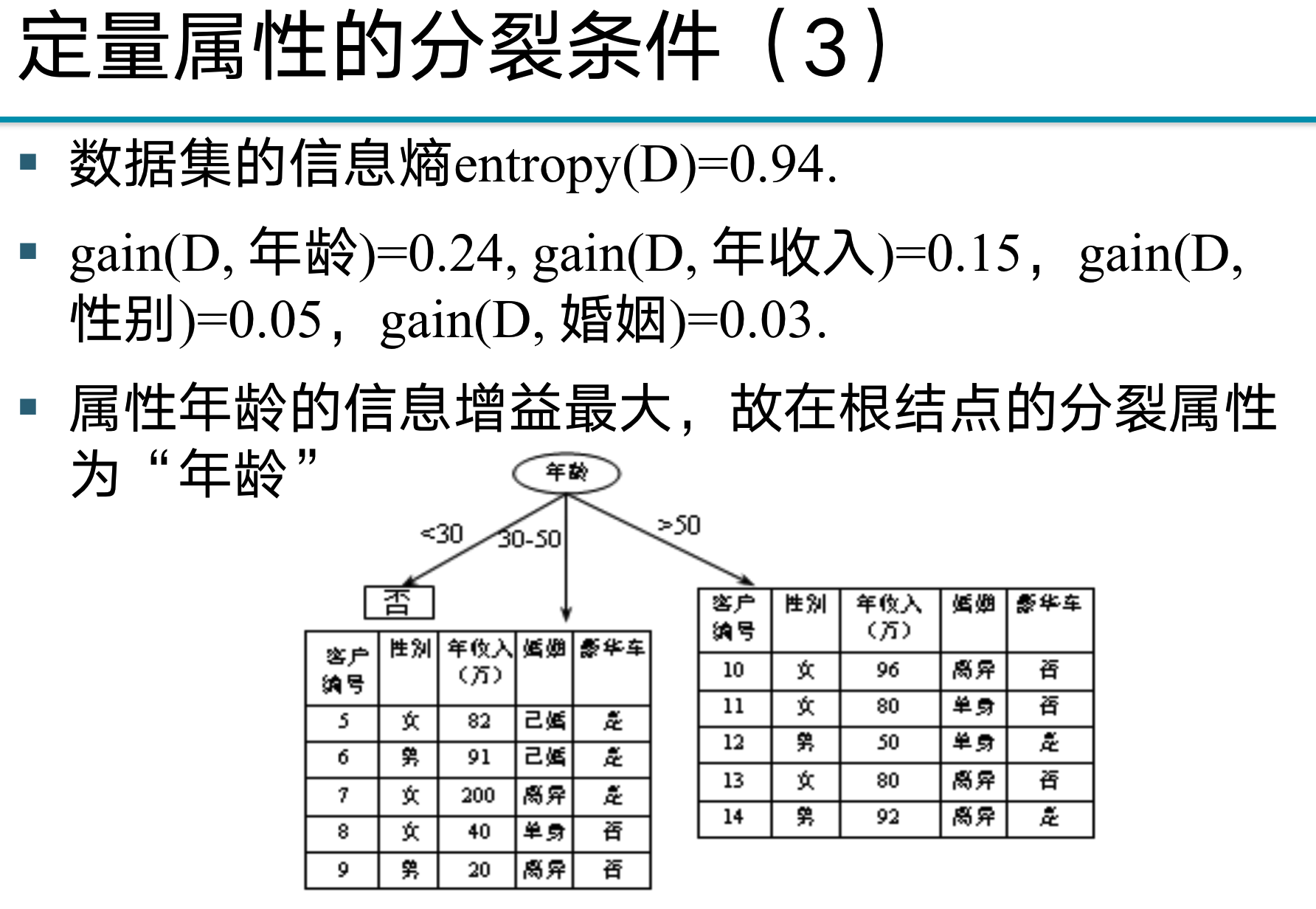
A simple example of playing basketball (vigilance) has been given above, and I probably feel it, because the above example has only two columns, one column is y (label), and the other column is x (feature), so I can’t understand the selection process of the decision tree , so use the following example to further introduce.

• in this example
  • The information entropy of the entire data set is calculated by luxury car
  • The calculation of qualitative data refers to the calculation according to the classification attribute x (such as marriage, gender, age here), that is, the information entropy before classification.
  • The calculation of quantitative data is to calculate the numerical attributes x (such as the annual income here), etc., and try to divide x into different classification conditions.
  • Information gain = information entropy before splitting - information entropy after splitting
  • By comparing the size, the greater the information gain (the more the information entropy decreases), it will become the splitting condition we choose

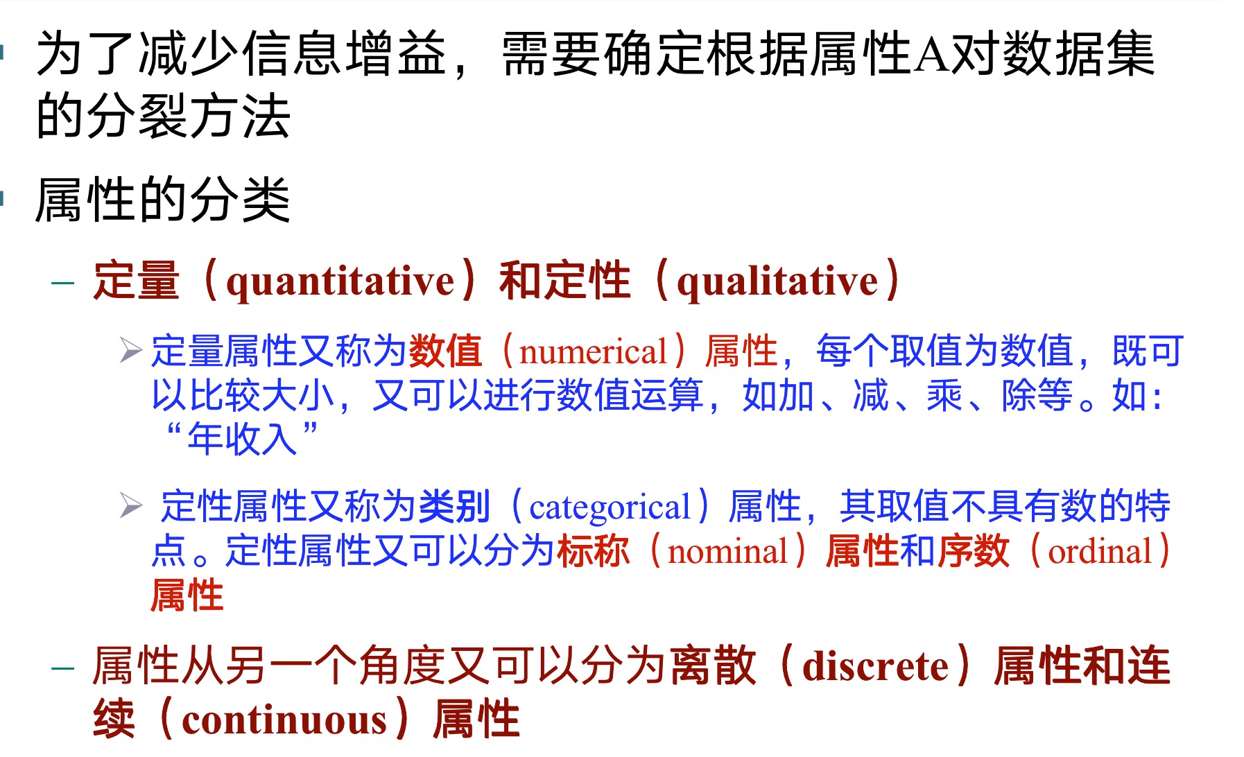
Qualitative (exam focus)

• Tips: For example, it is calculated by marriage here, that is, it is first divided into three situations: single, married, and divorced, and then each of them is calculated according to y (whether the luxury car is or not).

Quantitative

4.2 Naive Bayes classification

P41

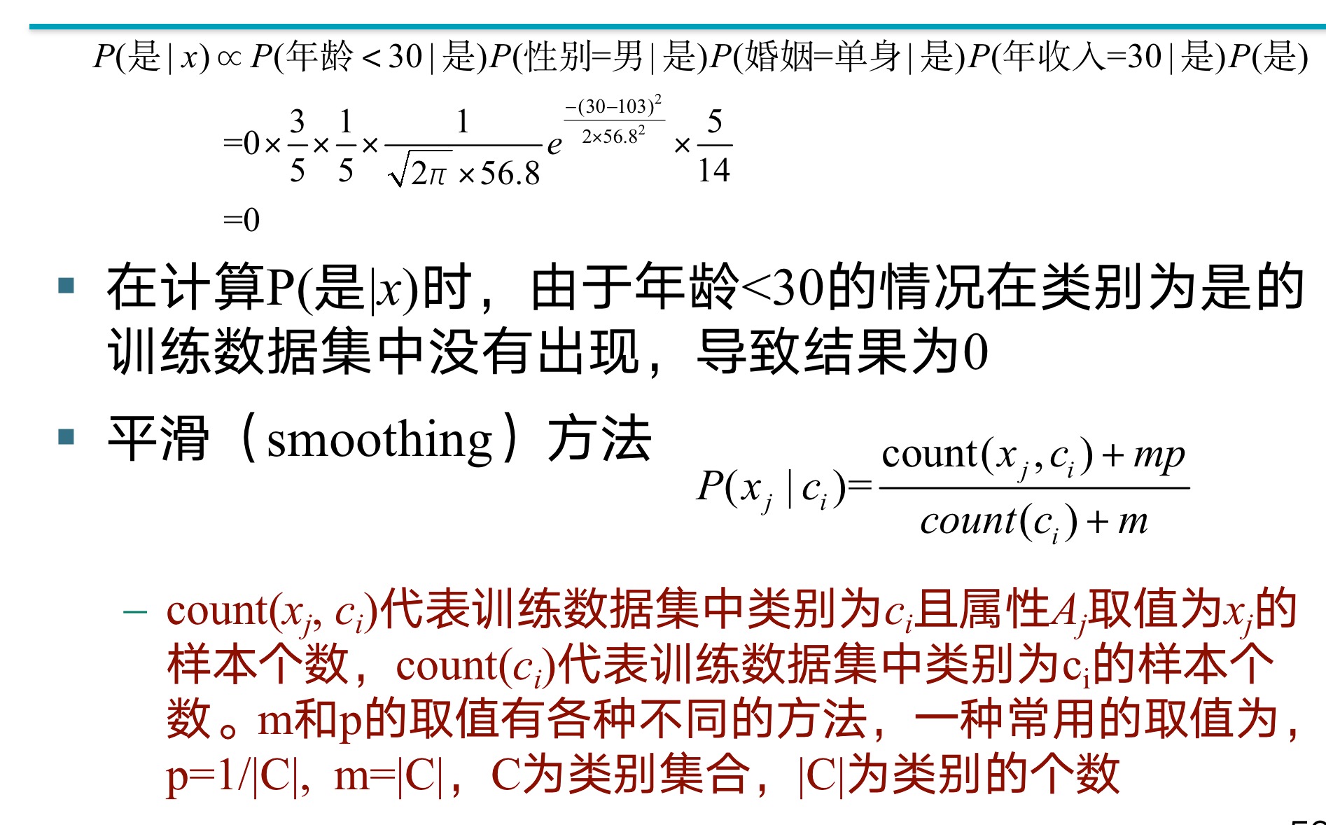
Smoothing is +1 per category

4.3 K nearest neighbor classification

• aggressive method

  • Decision Trees, Bayesian

• lazy method

  • K-Nearest Neighbors

• For a prediction sample, find the K samples most similar to it from the training data set, and use the category of these K samples to determine the category of this sample

• K is specified by the user. The selection method of similar samples depends on the method of measuring the similarity between samples. For the introduction of various similarity measuring methods, see Chapter 6

• After selecting K samples with the smallest distance to a test sample, you can use the voting method (voting) to count the number of samples in each category, and assign the majority of the K categories to the test sample

4.4 Measuring Classification Performance

4.4.1 Partitioning the dataset

• Holdout

  • Artificially determine the ratio of training data set and test data set, commonly used ratios are 2:1 and 1:1

• Cross-validation method (cross-validation)

  • Each sample is alternately used for training or testing set

  • n-fold cross-validation n-Folds cross-validation

  • Commonly used: 10-fold cross-validation

    • The data set is divided into 10 parts, each time using 9 points as the training set and 1 part as the test set

    • First, we split the dataset into 10 equal parts (10 samples each). Then, we perform 10 rounds of training and testing. In each round, we use 9 data (90 samples) to train our model and use the remaining 1 data (10 samples) to test the performance of the model. This way, each piece of data has one chance to be used as a test set, and the rest of the time it is used as a training set.

      In the end, we get 10 test scores, and we usually calculate their average as the final performance indicator. The advantage of this approach is that we use all the data for training and testing, and each sample is used once for testing.

  • Leave-one-out N-fold cross-validation

    • Leave-one-out is a special case of n-fold cross-validation, where n is equal to the total number of samples . That is, if we have 100 samples, we do 100 rounds of training and testing. In each round, we use 99 samples for training and the remaining one for testing.

      While this approach yields the least biased estimates, it is computationally expensive, especially when the sample size is very large. However, if the sample size is relatively small, this approach may be a good choice, as it allows us to make good use of all the data.

• Bootstrap

  • Bootstrapping uses sampling with replacement to construct the training dataset

4.4.2 Metrics

4.4.3 Comparison of Different Classification Models

• Gains chart (gains chart)

  • Gain plots are a visualization tool for showing the cumulative effect of model predictions. In the gain graph, the X-axis represents the proportion of samples (from the samples that are all predicted to be positive), and the Y-axis represents the proportion of positive samples.
  • The starting point of the gain map is (0,0) and the ending point is (1,1). If the model's predictions were perfectly accurate, the graph would be a graph of steps going up and to the right, where steps occur after all true examples are predicted as positive. If the model's predictions were not informative (ie, like random guessing), then the graph would be a diagonal line from (0,0) to (1,1).
  • Gain plots are a good way to evaluate how well a model predicts rankings, especially when we are more interested in predicting the ranking of positive samples than in the accuracy of the predictions.

• ROC curve

  • Y axis: the percentage of the number of positive samples contained in the sample in the total number of positive samples, that is, the true rate TP
  • X-axis: the proportion of negative samples in the selected sample to the total negative samples in the test sample, that is, the false positive rate FP
  • The starting point of the ROC curve is (0,0) and the ending point is (1,1). If the model's predictions are perfectly accurate, then the ROC curve will first go up to (0,1) and then to the right to (1,1). If the model's predictions are not informative, then the ROC curve will be a diagonal line from (0,0) to (1,1).
  • The area under the ROC curve (Area Under the ROC Curve, AUC) can be used as an indicator to measure the performance of the model. AUC values ​​range from 0.5 (no predictive power) to 1 (perfect prediction).

Chapter 5 Numerical Forecasting

5.1 Model checking

5.2 Nonlinear regression

How to Convert Nonlinear Regression to Linear Regression

1. For model $y=a{x}^b$ , after taking the logarithm becomes:$\log y=\log a+b\log x$.

2. For model $y=a{e}^{bx}$ , after logarithm, becomes:$\ln y=\ln a+bx$.

3. For the model $y=a+b\log x$ , if let$X=\log x$ , then the model becomes:$y=a+bX$.

These are common nonlinear models that can be transformed into linear models by logarithmic transformation or variable substitution. The advantage of this is that linear models are easier to handle both in theory and in practice.

5.3 Regression tree and model tree

SDR (Standard Deviation Reduction), information entropy, and information gain (Information Gain) are all criteria used to select split attributes in decision trees, but their applicable problems and specific calculation methods are different.

1. SDR（Standard Deviation Reduction）：

   SDR is used in decision trees for regression problems , that is, the target variable is a continuous value. It selects split attributes based on the standard deviation of the target attribute values . If a split can result in a significant drop in the standard deviation of the subdataset, then the split is probably good. Standard deviation is an indicator to measure the degree of dispersion of values ​​in a data set. The smaller the standard deviation, the more concentrated the data.

   The calculation formula of SDR is usually: $SDR=sd(D)-(|D1|/|D|)\ast sd(D1)-(|D2|/|D|)\ast sd\left(D2\right)$ . where$sd\left(D\right)$ represents the standard deviation of the target attribute value in the data set D,$|D|$ represents the number of samples contained in the data set D.

2. Information entropy and information gain (Information Gain) :

   Information entropy and information gain are used in decision trees for classification problems, that is, the target variable is discrete. Information entropy is a measure of data uncertainty, the greater the information entropy, the greater the uncertainty of the data. The information gain is an index to judge the importance of an attribute in the classification problem. The greater the information gain, the greater the contribution of this attribute to the classification.

   The calculation formula of information gain is: $Gain=Entropy(D)-\sum (|Di|/|D|)\ast Entropy\left(Di\right)$ Meanwhile,Entropy ( D ) Entropy$($$D$$)$$Entropy\left(D\right)$ is the information entropy of data set D,$|Di|/|D|$ is the proportion of sub-dataset Di in D.

In general, both SDR and information gain are indicators to evaluate the effectiveness of splitting attributes, but SDR is mainly used for regression problems, while information gain is mainly used for classification problems . They all try to find those attributes that can minimize the uncertainty as splitting attributes.

Chapter 6 Clustering

6.1 Classification of clustering methods

• Partitioning approach:
  • k-means, k-medoids and other methods.
• Hierarchical approach:
  • Agglomerative hierarchical clustering and divisive hierarchical clustering
  • Diana、 Agnes、BIRCH、 ROCK、CAMELEON等。
• Density-based approach
  • DBSCAN, OPTICS and DenClue etc.
• Model-based approach (Model-based)
  • EM, SOM and COBWEB, etc.

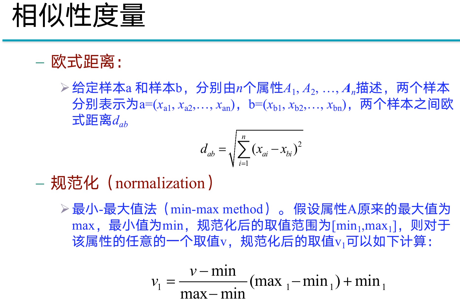
6.2 Similarity measurement method

Distance-Based Similarity Measures

cosine similarity

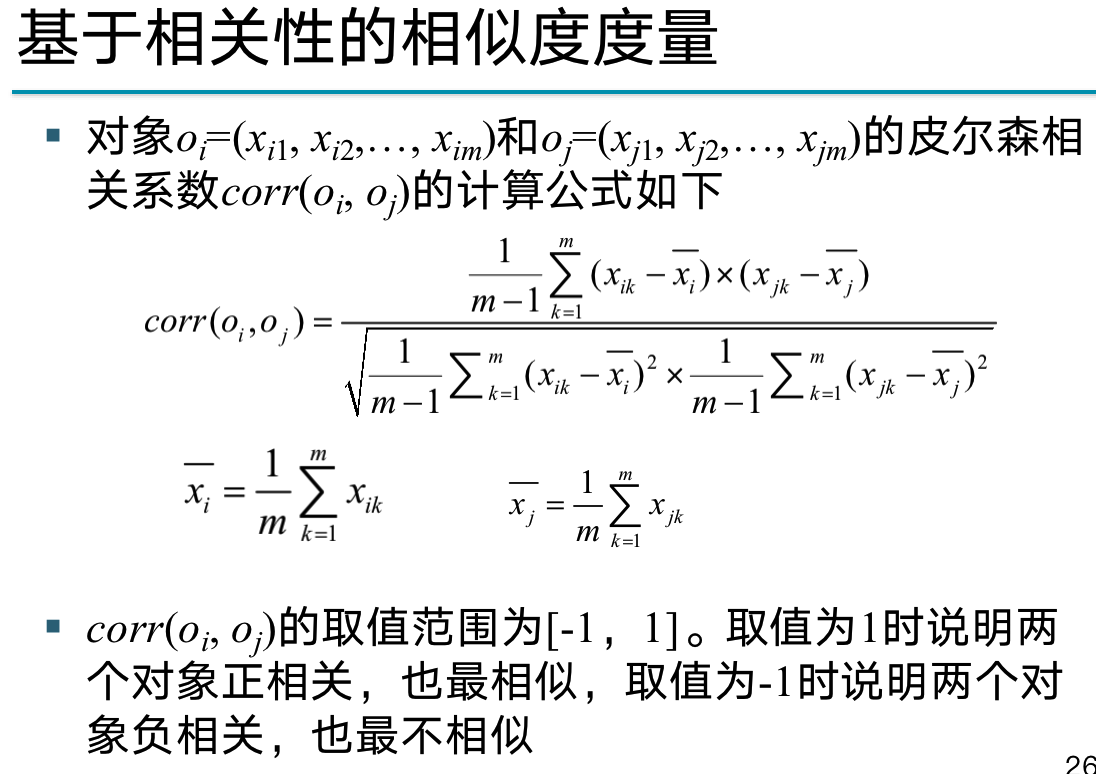
Correlation-Based Similarity Measures

Jaccard coefficient

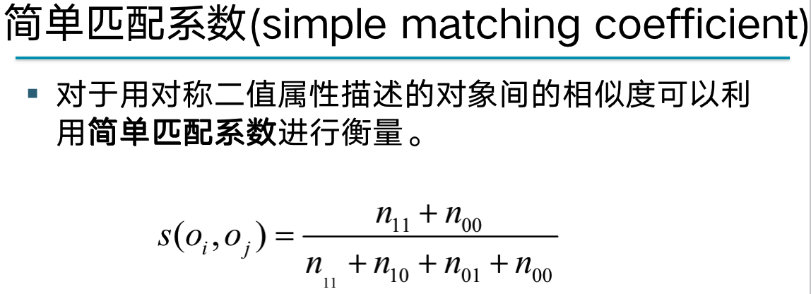
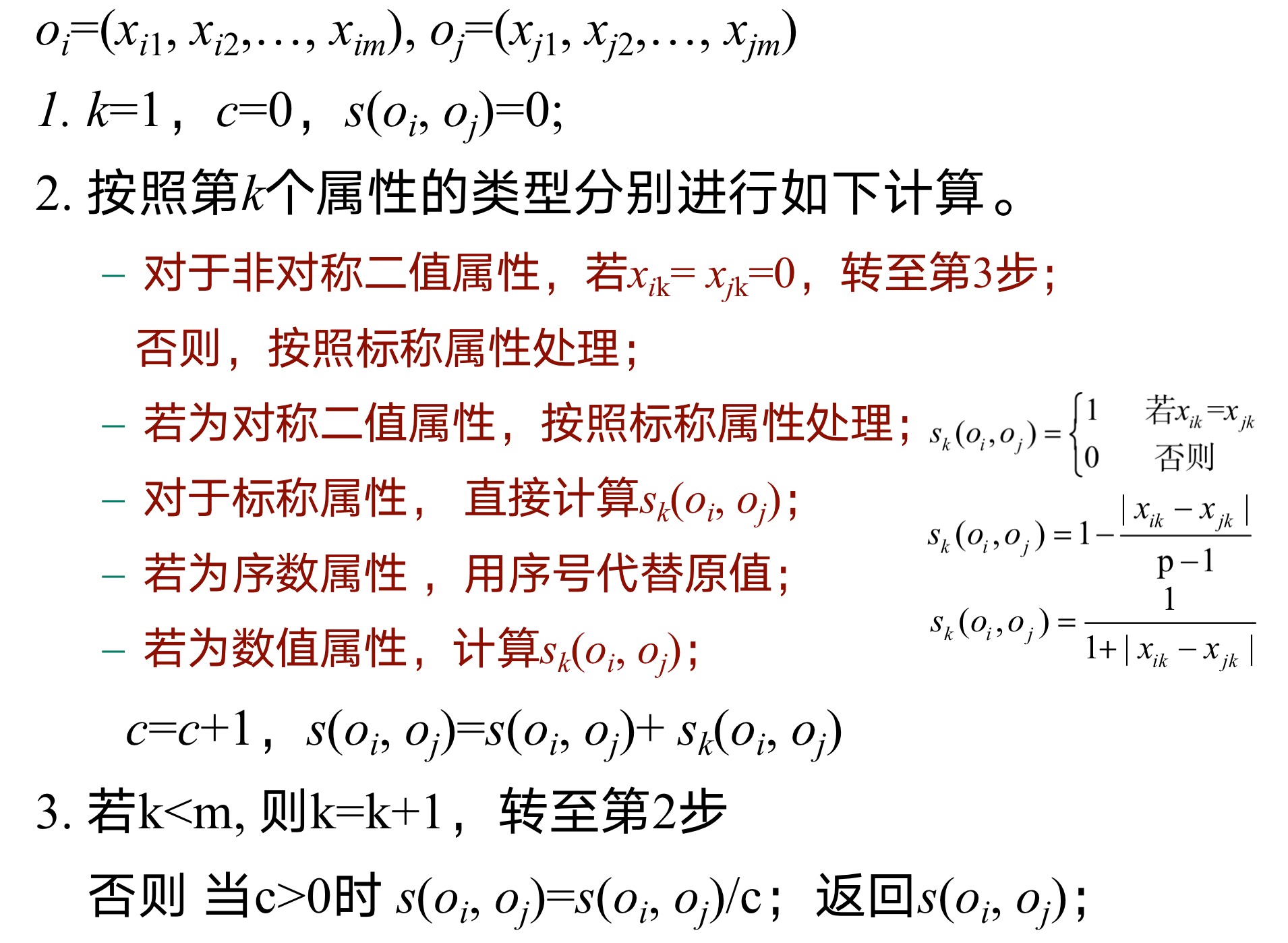
A Comprehensive Measure of Similarity of Heterogeneous Attributes

• Nominal means "relating to a name", and the value of the nominal attribute is some symbol or the name of a thing.

6.3 K-Means Clustering

• Calculate centroid
• 

Suppose we have a 2D dataset with six points: (1,1), (1,2), (2,1), (5,4), (5,5) and (6,5) , and we want to cluster these points into two categories, the following is a basic process of K-means clustering:

1. Initialization : First, we need to choose K (here K=2) initial centers (called centroids). There are various ways to choose the initial centroids, one of the simple ways is to randomly select K samples from the dataset. Suppose we choose (1,1) and (5,4) as the initial two centroids.

2. Assign to nearest centroid : Next, we assign each data point to the nearest centroid. This "nearest" is determined according to some distance metric, usually Euclidean distance. For our example, (1,1), (1,2) and (2,1) would be assigned to the first centroid, and (5,4), (5,5) and (6,5) would be assigned to assigned to the second centroid.

3. Recalculate the centroids : Then we need to recompute the centroids for each class. The centroid is the mean of all points it contains. For our example, the new centroid of the first class is ((1+1+2)/3, (1+2+1)/3) = (1.33, 1.33) and the new centroid of the second class is ( (5+5+6)/3, (4+5+5)/3) = (5.33, 4.67).

4. Repeat steps 2 and 3 : We keep repeating steps 2 and 3 until the centroid no longer changes significantly, or the preset maximum number of iterations is reached. In our case, the centroid has not changed anymore, so the algorithm stops here.

The final result is that (1,1), (1,2) and (2,1) are clustered into one category, and (5,4), (5,5) and (6,5) are clustered into another kind. Note that the result of K-means clustering may be affected by the selection of the initial centroid, and may fall into a local optimum. Therefore, in practice, it may be necessary to run the algorithm multiple times to select the best result.

6.4 Comparison of characteristics of various clustering methods

1. K-means (K-means):

advantage:

• The calculation speed is fast, and the efficiency on large-scale data sets is high.
• The output is easy to understand, and the clustering effect is moderate.

shortcoming:

• The number K of clusters needs to be set in advance, which is a challenge in many cases.
• Sensitive to the choice of initial centroid, may fall into local optimum.
• Works poorly for non-spherical (non-convex) data structures, and for clusters with large differences in size.
• Sensitive to noise and outliers.

Applicable scene:

• Suitable for continuous numerical data, not suitable for categorical data (use k-modes or k-prototype for extension).
• It performs better when the amount of data is large and the data dimension is relatively low.

2. Hierarchical Clustering:

advantage:

• There is no need to pre-set the number of clusters.
• The resulting hierarchical structure can be analyzed at different levels, suitable for hierarchical data.
• When the amount of data is not particularly large, the effect is often better than K-means.

shortcoming:

• The computational complexity is high, and it is difficult to handle large-scale data sets.
• Once a sample is classified into a certain class, it cannot be changed, which may lead to limited clustering effect.
• Sensitive to noise and outliers.

Applicable scene:

• When you need to get the hierarchical structure of the data.
• When the dataset is relatively small and has a significant hierarchy.

Supplement: A measure of the similarity between calculation clusters

1. Minimum distance (minimum distance), that is, single link Single link: Based on the minimum distance between nodes from two clusters to measure the similarity of two clusters,
2. The maximum distance (maximum distance), that is, the full link complete link: based on the maximum distance between the nodes from the two clusters to measure the similarity of the two clusters
3. The average distance (average distance), that is, the link Single link: based on the average distance between the nodes from the two clusters to measure the similarity of the two clusters
4. The average distance (average distance), that is, the link Single link: calculate the distance between the centroids of the two clusters to measure the similarity of the two clusters

3. DBSCAN (Density-Based Spatial Clustering of Applications with Noise)：

advantage:

• There is no need to pre-set the number of clusters.
• Cluster structures of arbitrary shapes can be discovered.
• It has the ability to identify noise points.

shortcoming:

• For datasets with non-uniform density, it may be difficult to find suitable parameters (such as density threshold).
• The clustering effect on high-dimensional data is usually not good.

Applicable scene:

• When clusters in a dataset take on complex shapes.

• When there are noise points or outliers in the data set.

• When the size and density of the dataset is relatively moderate, and the data dimensionality is not particularly high.

• Clustering effect measurement method

  • Cohesion (cohesion): measures the closeness of each object in the cluster

  • Separation (separation): Measures the degree of dissimilarity of objects between clusters

Chapter 8 Data Preprocessing

8.1 Data normalization

• Data normalization is also known as standardization
  • Min-max normalization
    • 
  • z-score
    • $Z=(X-m)/p$
    • 

8.2 Data discretization

• Equal distance binning, equal frequency binning
  • 
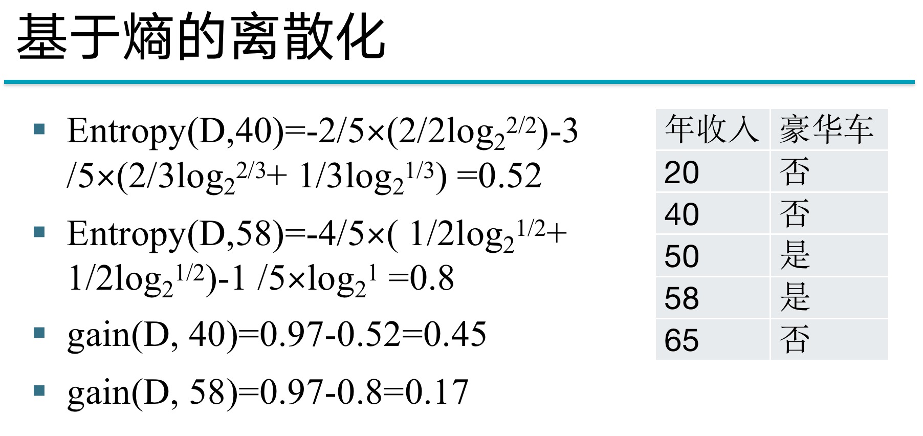
• Entropy-based discretization
  • Binning discretization is an unsupervised discretization method
  • Entropy-based discretization methods are commonly used supervised discretization methods
  • The smaller the value of information entropy, the purer the class distribution, and vice versa
  • 
• Discretization method ChiMerge
  • If entropy-based methods can be seen as top-down splitting methods, ChiMerge is a bottom-up merging method
  • ChiMerge starts from the fact that each value is a small interval, and continuously merges adjacent intervals to form a large interval. It is realized based on the statistical chi-square test

ChiMerge is a supervised discretization method based on the chi-square statistic for converting continuous variables into discrete variables. The basic principle of the ChiMerge method is to divide the range of continuous variables into a series of disjoint intervals, so that the distribution of the target variable corresponding to the value in the same interval is as consistent as possible, while the distribution of the target variable corresponding to different intervals is as different as possible.

The following are the basic steps of the ChiMerge method:

1. Initialization: Treat each value of the continuous attribute as a separate interval.

2. Computes the chi-square value for each pair of adjacent intervals.

3. Merge adjacent intervals with the smallest chi-square values, the merging of these two intervals does not significantly change the distribution of the target variable.

4. Repeat steps 2 and 3 until the chi-square values ​​of all adjacent intervals are greater than the preset threshold, or reach the preset number of intervals.

Below is a simple example. Suppose we have the following data:

Age	Class
23	+
45	-
56	+
60	-
33	+
48	-
50	-
38	+

We want to discretize Age using the ChiMerge method and Class is the target variable.

The steps to calculate the chi-square value are as follows:

1. For each pair of adjacent intervals, count the occurrences of the target categories '+' and '-' in each interval, respectively. For example, there is 1 occurrence of '+' and 0 occurrences of '-' in the first interval [23], and 0 occurrences of '+' and 1 occurrence of '-' in the second interval [45].

2. Construct a 2x2 observation frequency table, the row represents the interval, the column represents the category, and the cell value is the corresponding occurrence number.

   	‘+’	‘-’
   23	1	0
   45	0	1

3. From the observed frequency table, calculate the expected frequency for each cell. The expected frequency is the total number in the corresponding row multiplied by the total number in the corresponding column, then divided by the total observed frequency. In this example, all cells have an expected frequency of 0.5.

4. Calculate the chi-square value of each cell, which is (observed frequency - expected frequency)^2 / expected frequency, and then add up the chi-square values ​​of all cells to obtain the chi-square value of this pair of intervals. In this example, the chi-square value is (1-0.5)^2/0.5 + (0-0.5)^2/0.5 + (0-0.5)^2/0.5 + (1-0.5)^2/0.5 = 2 .

5. Perform this calculation for all adjacent intervals, find a pair of intervals with the smallest chi-square value, and then merge the pair of intervals.

In general, ChiMerge is an effective discretization method, especially suitable for those cases where the relationship between continuous variables and target variables is complex.

8.3 Data cleaning

• Handling missing data, handling noisy data, and identifying and handling data inconsistencies

• Dealing with Missing Data

  • If the dataset contains categorical attributes, a simple way to fill in missing values ​​is to assign the mean of the attribute values ​​of objects belonging to the same class to the missing value; for discrete or qualitative attributes, replace the mean with the mode

  • A more complex approach, which can be converted to a classification problem or a numerical prediction problem

Chapter 10 Data Warehouse

10.1 Related Concepts of Data Warehouse

• What is a data warehouse?
  • A data warehouse is a subject-oriented, integrated, time-varying, and stable collection of data used to support organizational decision-making.
• Why build a data warehouse?
  • There are redundancy and inconsistencies in the data in different systems. Each system only reflects a part of the information and is not related to each other, forming an information island.
  • Directly accessing the operational system to obtain data for analysis will inevitably interfere with the efficient operation of things in the operational system and affect the efficiency of business operations.
• The difference between data warehouse and data mart
  • database:
    • 1. It is generally created before the data mart.
    • 2. A variety of different data sources.
    • 3. Include all detailed data information.
    • 4. The data content is at the company level, without specific topics or fields.
    • 5. It conforms to the third normal form.
    • 6. It is usually necessary to optimize how to process massive data.
  • Data mart:
    • 1. Generally, after the data warehouse is created.
    • 2. The data warehouse is the data source.
    • 3. Contains moderately aggregated data and some detailed data.
    • 4. The data content is at the departmental level, with specific fields.
    • 5. Star shape and snowflake shape.
    • 6. Usually pay more attention to how to quickly access and analyze.

10.2 Architecture of Data Warehouse

• Architecture of Data Warehouse System
  • 
  • Metadata is the descriptive information of the data in the data warehouse. It mainly describes three aspects of information: data source data information, data extraction and conversion information, and data information in the data warehouse.

10.3 Multidimensional Data Model

• What is a multidimensional data model?
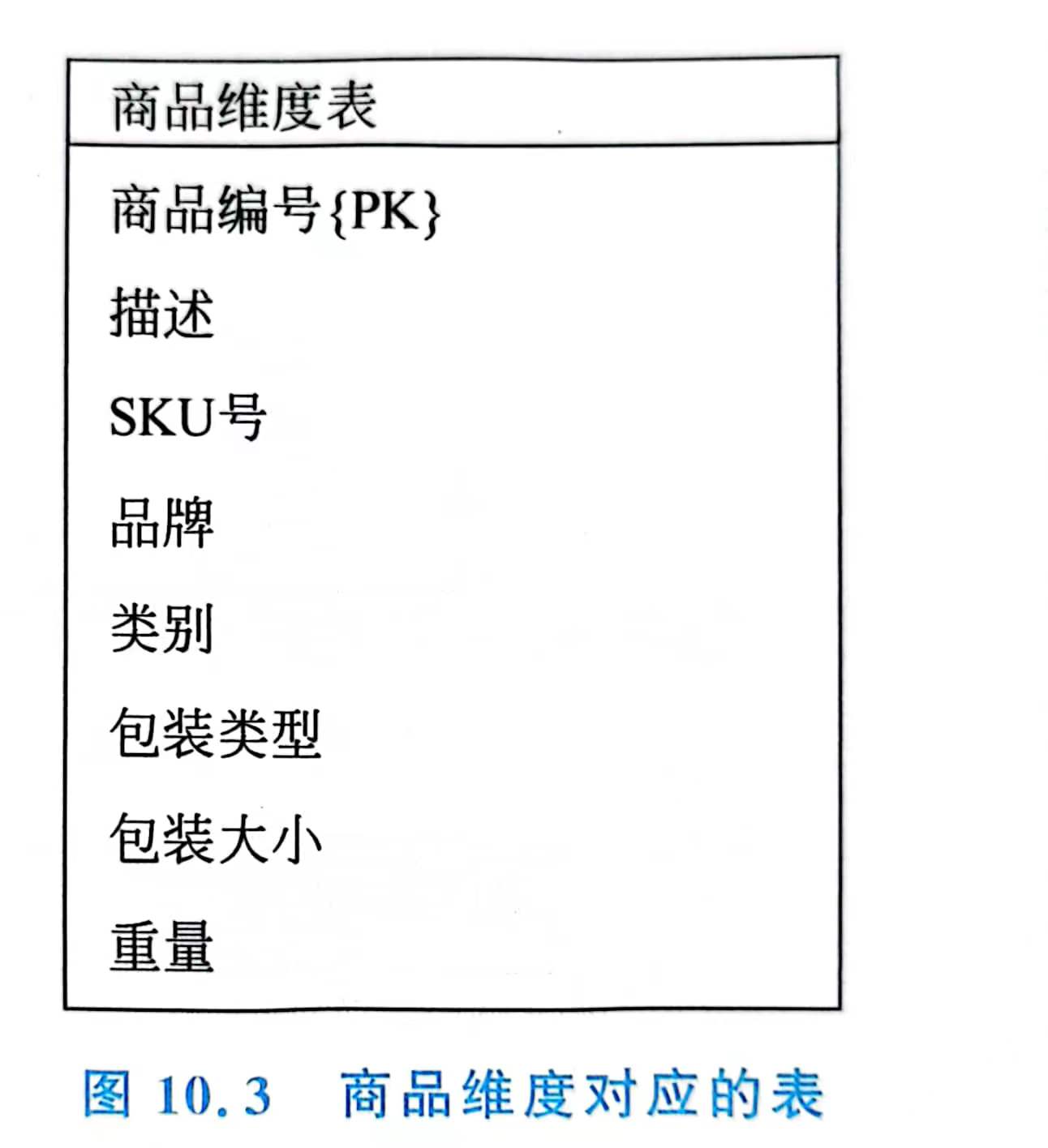
  • The multidimensional data model, also known as the dimensional data model, consists of dimension tables and fact tables.
• fact sheet
  • 
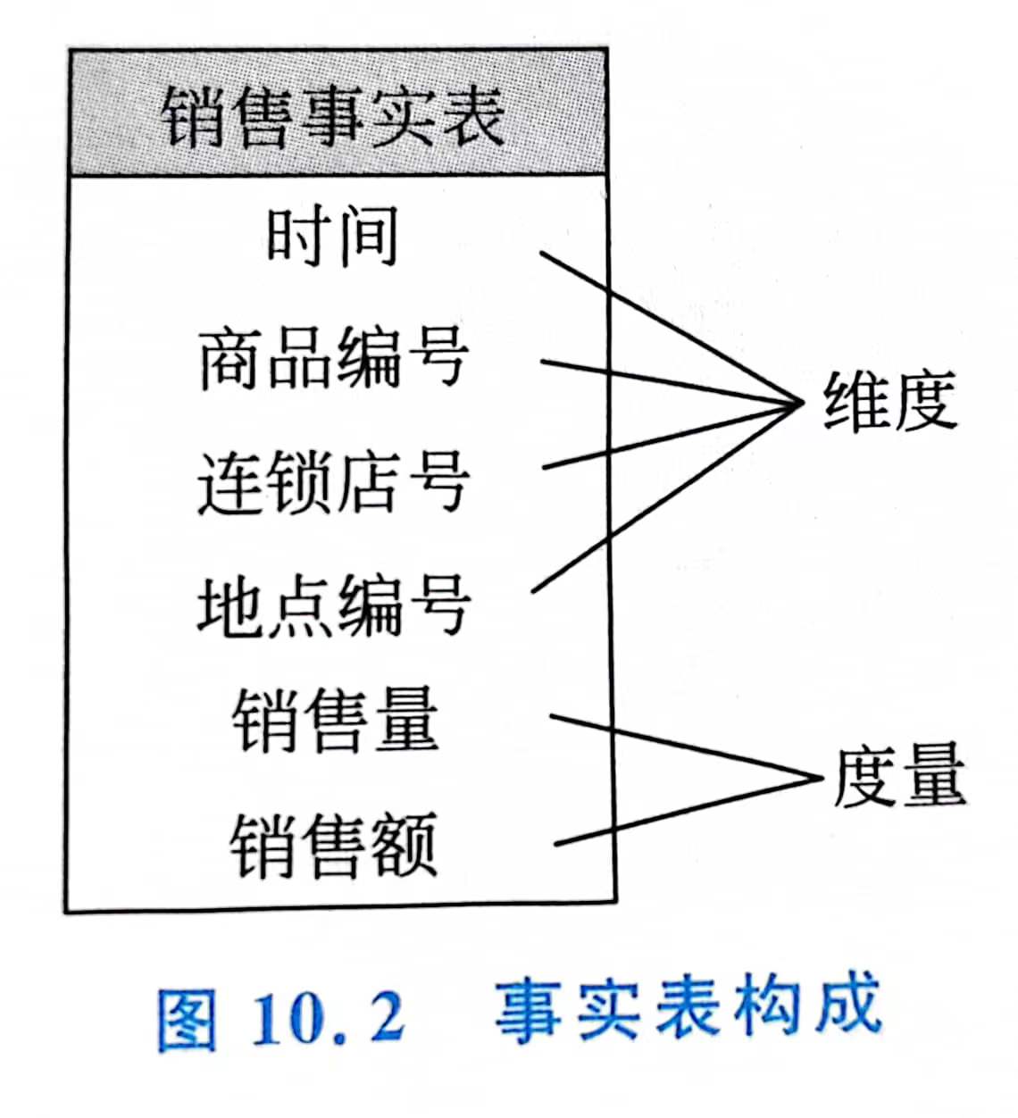
  • Metrics are usually quantitative attributes and are stored in fact tables. Metrics are preferably additive.
• dimension table
  •