Table of contents
Matplotlib is a two-dimensional plotting library for Python , used to generate various graphics that meet publication quality or cross-platform interactive environments .

Zero, graphic analysis and workflow
0.1 Graphic analysis
0.2 Workflow
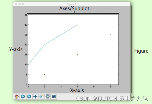
Matplotlib PlottingThe basic steps are generally 6 steps, which are: 1- preparing data , 2- creating graphics , 3- drawing , 4- customizing settings , 5- saving graphics , 6- displaying graphics .
>>> import matplotlib.pyplot as plt
>>> x = [1,2,3,4]
>>> y = [10,20,25,30]
# 步骤1
>>> fig = plt.figure()
# 步骤2
>>> ax = fig.add_subplot(111)
# 步骤3
>>>ax.plot(x,y,color='lightblue',linewidth=3)
# 步骤4、5
>>> ax.scatter([2,4,6], [5,15,25], color='darkgreen', marker='^')
>>> ax.set_xlim(1, 6.5)
>>> plt.savefig('foo.png')
>>> plt.show()
# 步骤6
The above code is explained below:
Step 1 Create a new Figure object .plt.figure() Returns a new, empty drawing area into which graphical elements can be added.
Step 2 Add a subgraph on the Figure . fig.add_subplot(111) Adds an Axes object containing a single subplot . The parameter (111) here means **Divide the entire drawing area into a grid of 1 row and 1 column, and select the first subplot**.
Step 3 draws a line graph on the subplot .ax.plot(x, y, color=‘lightblue’, linewidth=3) Draws a line using the given x and y values , the specified line color is light blue , and the line width is 3 .
Steps 4 and 5 add a scatterplot on the subplot . ax.scatter([2,4,6], [5,15,25], color='darkgreen', marker='^') at coordinates (2, 5), (4, 15), (6, 25 ) placeadd three scatters, which is dark green in color and triangular in shape.
Steps 4 and 5 also call the ax.set_xlim() method to set the display range of the x-axis from 1 to 6.5 to suit the display of data and scatter points.
Step 6 Save the graphic as an image file . plt.savefig('foo.png') saves the current figure as a picture file named "foo.png" .
The last step displays the graph .plt.show()Display the graph in a pop-up window. After finishing the whole drawing process, save the graphic as "foo.png" and display it in the window at the same time.
1. Prepare data
1.1 One-dimensional data
we firstGenerate a one-dimensional array of length 100 using the Numpy library, to get familiar with Matplotlib step by step through its operation.
# 导入 NumPy 库并将其命名为 np
>>> import numpy as np
# 使用 np.linspace() 函数生成一个从 0 到 10(包含)的等间距数组,数组长度为 100。生成一个长度为 100 的一维数组,并将其赋值给变量 x
>>> x = np.linspace(0, 10, 100)
>>> y = np.cos(x)
>>> z = np.sin(x)
1.2 Two-dimensional data or pictures
Now that we have some understanding of Matplotlib, let's useNumPyandMatplotlib libraryLet's generate some data and images.
>>> data = 2 * np.random.random((10, 10))
# 生成一个形状为(10, 10)的随机数组,其中的元素取值范围在0到2之间,并将结果存储在变量data中
>>> data2 = 3 * np.random.random((10, 10))
# 创建一个形状为(10, 10)的随机数组,元素的取值范围在0到3之间
>>> Y, X = np.mgrid[-3:3:100j, -3:3:100j]
#  创建两个二维数组Y和X,分别包含了从-3到3之间的100个等间隔的值
>>> U = -1 - X**2 + Y
# 计算一个与X和Y相关的二维数组U
>>> V = 1 + X - Y**2
# 计算另一个与X和Y相关的二维数组V
>>> from matplotlib.cbook import get_sample_data
# 导入函数get_sample_data,用于获取示例数据文件的路径
>>> img = np.load(get_sample_data('axes_grid/bivariate_normal.npy'))
# 加载一个示例数据文件,存储二维数组img
2. Draw graphics
Matplotlib is a Python library for drawing charts and visualizing data . passimport matplotlib.pyplot module, we can use the functions in it to create and display charts . It is usually named plt to simplify the amount of typing used in the code.
>>> import matplotlib.pyplot as plt
# 导入了Matplotlib库,并将其命名为plt
2.1 Canvas
By calling the plt.figure() function andspecify the appropriate parameters, we can create Figure objects of different sizes to draw charts and graphs on them.
>>> fig = plt.figure()
# 创建一个Figure对象并将其赋值给变量fig
>>> fig2 = plt.figure(figsize=plt.figaspect(2.0))
# 创建另一个Figure对象并将其赋值给变量fig2
2.2 Coordinate axes
Graphics are based onAxisDrawn for the core , in most cases submaps will suffice.The subplot is the axis of the grid system。
By calling the add_subplot() method of the Figure object or using the subplots() function , we canCreate multiple subplots or axes on a Figure and assign them to different variables, so that something different is drawn on each subplot.
>>> fig.add_axes()
# 调用Figure对象的add_axes()方法,用来手动添加一个新的坐标轴到图形上
>>> ax1 = fig.add_subplot(221) # row-col-num
# 使用add_subplot()方法在Figure对象上创建一个子图(Axes对象)
# 参数(221)表示将整个图形窗口划分为2行2列的子图网格,并选择第一个子图作为当前的绘图区域(ax1)
>>> ax3 = fig.add_subplot(212)
# 使用add_subplot()方法在Figure对象上创建另一个子图(Axes对象)
# 参数(212)表示将整个图形窗口划分为2行1列的子图网格,并选择第二个子图作为当前的绘图区域(ax3)
>>> fig3, axes = plt.subplots(nrows=2,ncols=2)
# 使用subplots()函数创建一个有多个子图的Figure对象(fig3),并将两个返回值分别赋值给fig3和axes
# 参数nrows和ncols分别指定了子图的行数和列数,生成了一个2行2列的子图网格
>>> fig4, axes2 = plt.subplots(ncols=3)
# 使用subplots()函数创建另一个有多个子图的Figure对象(fig4),并将两个返回值分别赋值给fig4和axes2
# 参数ncols指定了子图的列数,生成了一个1行3列的子图网格
3. Drawing routine
3.1 One-dimensional data
we can alsoDraw different types of graphs and charts using the Matplotlib library。
>>> fig, ax = plt.subplots()
# 创建了一个Figure对象(fig)和一个Axes对象(ax)
# Figure对象代表整个图形窗口,而Axes对象代表一个具体的绘图区域,我们可以在其上绘制各种图形和图表
>>> lines = ax.plot(x,y) # 用线或标记连接点
# 使用plot()函数在Axes对象上绘制了一条线,通过连接给定的点(x, y)
>>> ax.scatter(x,y) # 缩放或着色未连接的点
# 使用scatter()函数在Axes对象上绘制散点图,展示了未连接的点
>>> axes[0,0].bar([1,2,3],[3,4,5]) # 绘制等宽纵向矩形
# 在子图网格中的第一个子图(axes[0, 0])上绘制了垂直的等宽条形图,通过指定x轴和对应的高度值来创建矩形条
>>> axes[1,0].barh([0.5,1,2.5],[0,1,2]) # 绘制等高横向矩形
# 在子图网格中的第二个子图(axes[1, 0])上绘制了水平的等高条形图,通过指定y轴和对应的宽度值来创建矩形条
>>> axes[1,1].axhline(0.45) # 绘制与轴平行的横线
# 在子图网格中的第三个子图(axes[1, 1])上绘制了与y轴平行的横线,通过指定y轴的值来定义水平位置
>>> axes[0,1].axvline(0.65) # 绘制与轴垂直的竖线
# 在子图网格中的第四个子图(axes[0, 1])上绘制了与x轴垂直的竖线,通过指定x轴的值来定义垂直位置
>>> ax.fill(x,y,color='blue') # 绘制填充多边形
# 使用fill()函数在Axes对象上绘制了填充多边形,通过连接给定的点(x, y)并填充指定的颜色
>>> ax.fill_between(x,y,color='yellow') # 填充y值和0之间
# 使用fill_between()函数在Axes对象上绘制了填充区域,通过将y值和0之间的区域填充成指定的颜色
3.2 Vector fields
Next, we continue to learnUse the Matplotlib library to add arrows and draw 2D arrow plots, can help us visualize vector fields and streamline diagrams very well .
>>> axes[0,1].arrow(0,0,0.5,0.5) # 为坐标轴添加箭头
# 在子图网格中的第四个子图(axes[0,1])上添加了一个箭头
>>> axes[1,1].quiver(y,z) # 二维箭头
# 在子图网格中的第三个子图(axes[1,1])上绘制了二维箭头图。quiver()函数用于绘制向量场,其中 y 和 z 是对应x轴和y轴上的向量分量
>>> axes[0,1].streamplot(X,Y,U,V) # 二维箭头
# 在子图网格中的第四个子图(axes[0,1])上绘制了二维箭头图。streamplot()函数用于绘制流线图,其中 X 和 Y 是等距离的点网格,U 和 V 是对应点上的向量分量
3.3 Data distribution
We can plot in Matplotlibhistogram、 box plotandViolin diagram, in order to visualize the distribution of the data and statistics such as outliers .
>>> ax1.hist(y) #直方图
# 在Axes对象 ax1 上绘制了直方图,图用于显示数据的分布情况。y 是要绘制直方图的数据
>>> ax3.boxplot(y) # 箱形图用于展示数据的概要统计信息,包括中位数、四分位数等,y 是要绘制箱形图的数据
>>> ax3.violinplot(z) # 小提琴图结合了箱形图和核密度估计图的特点,可以显示出数据的分布密度和范围,z 是要绘制小提琴图的数据
3.4 Two-dimensional data or pictures
The following is to use the Matplotlib library display image in graphics window, and configure it with the specified colormap and parameters .
>>> fig, ax = plt.subplots()
# 创建了一个Figure对象(fig)和一个Axes对象(ax),代表整个图形窗口以及绘图区域
>>> im = ax.imshow(img, cmap='gist_earth', interpolation='nearest', vmin=-2, vmax=2)
# 使用imshow()函数在Axes对象上显示图像
# img是要显示的图像数据,cmap参数指定了色彩表的名称(这里使用了'gist_earth'),interpolation参数指定了图像插值的方法,vmin和vmax参数用于设置图像的最小和最大值的范围
# 色彩表或RGB数组
Through the above settings, we canDisplay images using Matplotlib, and select the appropriate color table, interpolation method, and range of image values to present the image as required .
Next we use the Matplotlib library to draw different types of pseudocolor maps and contour lines :
>>> axes2[0].pcolor(data2) # 二维数组伪彩色图
# pcolor()函数用于绘制二维数组的伪彩色图,data2 是要绘制的数据
>>> axes2[0].pcolormesh(data) # 二维数组等高线伪彩色图
# pcolormesh()函数用于绘制二维数组的等高线伪彩色图,data 是要绘制的数据
>>> CS = plt.contour(Y,X,U)
# contour()函数用于绘制等高线图,Y 和 X 分别是数据点的横纵坐标,U 是对应的高度值。CS 是返回的等高线对象
>>> axes2[2].contourf(data1) # 等高线图
# contourf()函数用于绘制等高线图,并为区域着色,data1 是要绘制的数据
>>> axes2[2]= ax.clabel(CS) # 等高线图标签
# clabel()函数用于在等高线图上添加标签,CS 是等高线对象
By using these functions, we can draw a two-dimensional array of pseudo-color maps, contour pseudo-color maps and contour maps in Matplotlib , and perform image processingmore customization, such as adding tags.
4. Custom Graphics
4.1 Color, color bar and color table
You can also use the Matplotlib library to draw different types of line graphs and images, and make various customizations, such as setting colors, transparency, adding legends, etc.
>>> plt.plot(x, x, x, x**2, x, x**3)# 在当前Figure上绘制了三条线图
# plot()函数用于绘制线图,参数x表示X轴的数据,参数x, x2, x, x3 分别表示三条曲线的Y轴数据
>>> ax.plot(x, y, alpha = 0.4)
# 在Axes对象 ax 上绘制了一条线图,并设置了透明度为0.4
# alpha 参数用于控制线图的透明度,x 和 y 分别表示X轴和Y轴的数据
>>> ax.plot(x, y, c='k')
# 在Axes对象 ax 上绘制了一条线图,并设置了颜色为黑色
# c 参数用于设置线图的颜色,'k' 表示黑色,x 和 y 分别表示X轴和Y轴的数据
>>> fig.colorbar(im, orientation='horizontal')
# 在当前Figure上添加了一个水平方向的图例
# colorbar()函数用于添加图例,在这里将 im 对象作为参数传入,并指定了图例的方向为水平
>>> im = ax.imshow(img, cmap='seismic')
# 在Axes对象 ax 上显示了一张图像,并使用色彩表 'seismic' 进行渲染
# imshow()函数用于显示图像,img 是要显示的图像数据,cmap 参数指定了色彩表的名称
4.2 Marking
Use the Matplotlib library to create a Figure object and an Axes object, and draw scatter and line graphs.
>>> fig, ax = plt.subplots()# 创建了一个包含一个Axes对象的Figure对象
# 通过 fig 来控制整个图像窗口,通过 ax 来控制具体的绘图区域
>>> ax.scatter(x,y,marker=".")
# 在Axes对象 ax 上绘制了一组散点图
# scatter()函数用于绘制散点图,x 和 y 分别表示X轴和Y轴的数据,marker 参数指定了数据点的标记形状,这里使用 "." 表示小圆点
>>> ax.plot(x,y,marker="o")
# 在Axes对象 ax 上绘制了一条线图,同时每个数据点也被标记出来
# plot()函数用于绘制线图,x 和 y 分别表示X轴和Y轴的数据,marker 参数指定了数据点的标记形状,这里使用 "o" 表示实心圆
By using these functions, we can create Figure objects and Axes objects in Matplotlib , andDraw scatterplots and line plots on Axes objects, you can also customize the graphics in various ways, such as setting the shape and color of the marker.
4.3 Line type
useMatplotlib library draws line graphs, and make some customizations to the lines.
>>> plt.plot(x,y,linewidth=4.0)
# 绘制了一条线图,并设置了线条的宽度为4.0
# plot()函数用于绘制线图,x 和 y 分别表示X轴和Y轴的数据,linewidth 参数指定了线条的宽度
>>> plt.plot(x,y,ls='solid')
# 绘制了一条线图,并将线条样式设置为实线
# ls 参数用于设置线条的样式,'solid' 表示实线
>>> plt.plot(x,y,ls='--')
# 绘制了一条线图,并将线条样式设置为虚线
# ls 参数用于设置线条的样式,'--' 表示虚线
>>> plt.plot(x,y,'--',x**2,y**2,'-.')
# 绘制了两条线图,一条使用虚线样式,一条使用点划线样式
# 多个数据序列可以在同一个 plot() 函数中传入,使用不同的样式区分
# 这里先绘制了一条虚线样式的线图,再绘制了一条点划线样式的线图
>>> plt.setp(lines,color='r',linewidth=4.0)
# 用于设置已绘制线图的属性
# setp() 函数用于批量设置线条属性,lines 参数指定要设置的线条对象,color 参数设置线条的颜色为红色,linewidth 参数设置线条的宽度为4.0
4.4 Text and annotation
The text() and annotate() functions of the Matplotlib library are used to add text and annotations to the image .
>>> ax.text(1, -2.1,'Example Graph', style='italic')
# 在Axes对象 ax 上添加了一个文本标签
# text()函数用于在指定的坐标位置添加文本,第一个参数是X轴坐标,第二个参数是Y轴坐标,第三个参数是要显示的文本内容
>>> ax.annotate("Sine", xy=(8, 0), xycoords='data', xytext=(10.5, 0), textcoords='data', arrowprops=dict(arrowstyle="->",connectionstyle="arc3"),)
# 在Axes对象 ax 上添加了一个箭头和注释
# annotate()函数用于在图像中添加带有注释和箭头的文本,第一个参数是注释的文本内容,xy参数表示箭头尖端的坐标,xycoords参数表示xy坐标的类型,xytext参数表示注释文本的坐标,textcoords参数表示xytext坐标的类型
# 通过arrowprops参数可以设置箭头的样式和连接样式
4.5 Mathematical symbols
Set the title of the image using the title() function of the Matplotlib library :
>>> plt.title(r'$sigma_i=15$', fontsize=20)
# 设置了图像的标题为"σi=15",其中$...$表示使用LaTeX格式的数学公式进行显示。通过在字符串前加上r字符来指定该字符串为原始字符串,以便正确显示特殊字符
# fontsize=20参数用于设置标题的字体大小为20
4.6 Size restrictions, legend and layout
4.6.1 Size constraints and automatic adjustment
>>> ax.margins(x=0.0,y=0.1) # 添加内边距
>>> ax.axis('equal') # 将图形纵横比设置为1
>>> ax.set(xlim=[0,10.5],ylim=[-1.5,1.5]) # 设置x轴与y轴的限制
>>> ax.set_xlim(0,10.5) # 设置x轴的限制
4.6.2 Legend
>>> ax.set(title='An Example Axes', ylabel='Y-Axis', xlabel='X-Axis')
# 设置标题与x、y轴的标签
>>> ax.legend(loc='best')
4.6.3 Marking
# 手动设置X轴刻度
>>> ax.xaxis.set(ticks=range(1,5),ticklabels=[3,100,-12,"foo"])
# 设置Y轴长度与方向
>>> ax.tick_params(axis='y', direction='inout', length=10)
4.6.4 Subplot Spacing
# 调整子图间距
>>> fig3.subplots_adjust(wspace=0.5,hspace=0.3,left=0.125, right=0.9, top=0.9, bottom=0.1)
# 设置画布的子图布局
>>> fig.tight_layout()
4.6.5 Coordinate axis edge
>>> ax1.spines['top'].set_visible(False)
# 隐藏顶部坐标轴线
>>> ax1.spines['bottom'].set_position(('outward',10))
# 设置底部边线的位置为outward
5. Save
5.1 Save Canvas
Use the savefig() function of the Matplotlib library to save the current image as a PNG file named "foo.png" .
>>> plt.savefig('foo.png')
# 使用savefig()函数将当前绘制的图像保存为一个PNG文件。'foo.png'是保存的文件名,可以根据需要修改为其他文件名,例如'result.png'
5.2 Save transparent canvas
Use the savefig() function of the Matplotlib library to save the current image as a PNG file named "foo.png" with a transparent background .
>>> plt.savefig('foo.png', transparent=True)
# 使用savefig()函数将当前绘制的图像保存为一个PNG文件,并通过将transparent参数设置为True来实现透明背景
# 'foo.png'是保存的文件名,可以根据需要修改为其他文件名,例如'result.png'
6. Display graphics
Use the show() function of the Matplotlib library to display the currently plotted image :
>>> plt.show()
# 调用show()函数,它将当前绘制的图像显示在屏幕上
# 这个函数会打开一个图形窗口,并在其中显示图像
by usingshow() function, you can display the image drawn by Matplotlib.
7. Closing and Clearing
Use three functions of the Matplotlib library to clear the image or close the window
>>> plt.cla() # 清除坐标轴
# 调用cla()函数,它会清除当前坐标轴的内容
>>> plt.clf() # 清除画布
# 调用clf()函数,它会清除整个当前图像的内容,包括坐标轴和所有绘制的内容
>>> plt.close() # 关闭窗口
# 调用close()函数,它会关闭当前图像的窗口
By using these functions, we can clear the contents of the current image or close the image window . But it should be noted that,The cla() and clf() functions do not directly affect the display of the image window, but instead clears the contents of the image or axes ,The close() function will close the image window。