Hessian matrix and Jacobian matrix understanding

---

---

Personal notes:

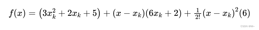
1: Unary Taylor expansion formula

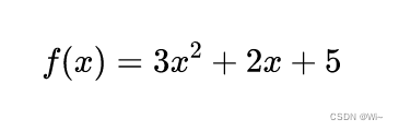
Example: f(x) = 3x² + 2x + 5 Taylor expansion at x=0 or x=1

When x=0:

When x=1:

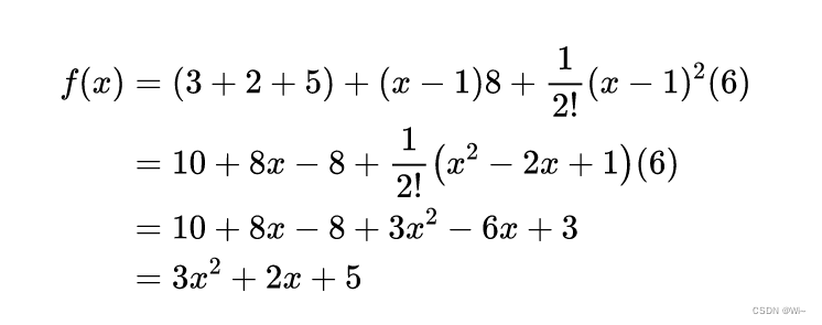
No matter how much Xk is equal to, the sum of the final expanded formulas is equal to f(x) = 3x² + 2x + 5

2: Binary Taylor expansion formula

Taylor expansion of x and y at k:

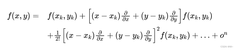
simplified:

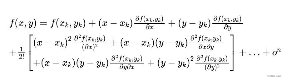
Simplification:
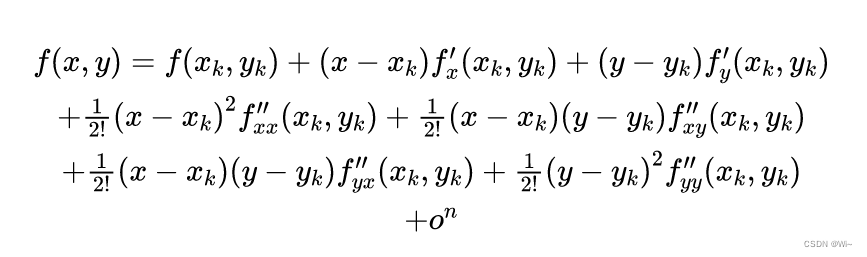①
$f_{xx}^{\prime \prime }$is taking two derivatives with respect to x.

②
$f_{xy}^{\prime \prime }$It is to take a derivative with respect to x first, and then take a derivative with respect to y.

③
$f_{yx}^{\prime \prime }$It is to take a derivative with respect to y first, and then take a derivative with respect to x.
(where ③ = ②)

④
$f_{yy}^{\prime \prime }$is taking the derivative of y twice.

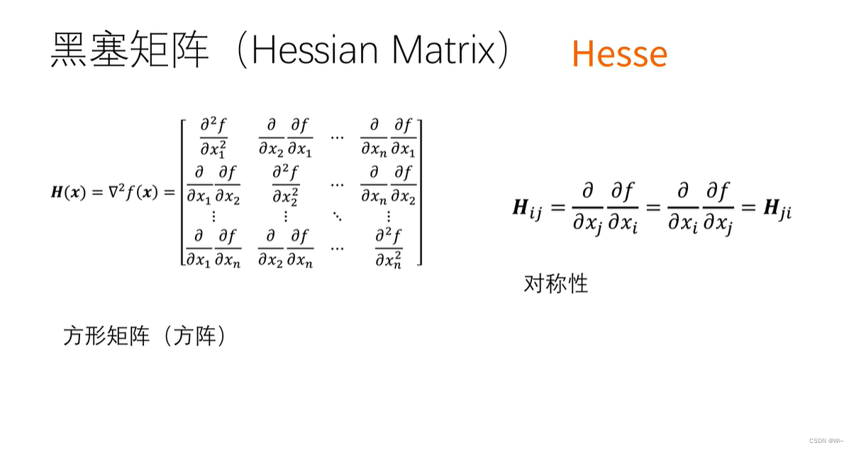
3: Hessian matrix of binary functions

Binary function point $f(x_1,x_2)$ at$X^{(k)}(x_1^{(k)},x_2^{\left(k\right)})$ at the Taylor expansion is:

where $\Delta x{\_}_1$ = $x_1$ − $x_1^{\left(k\right)}$, $\Delta x{\_}_2$ = $x_2$ − $x_2^{\left(k\right)}$

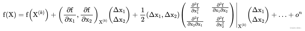
Right now:

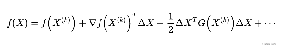
(1): where

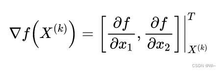
it is $f\left(X\right)$ at$X^{\left(k\right)}$ Gradient at point.

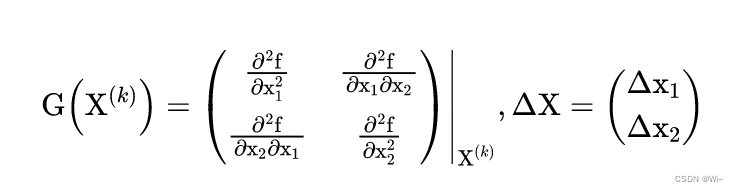
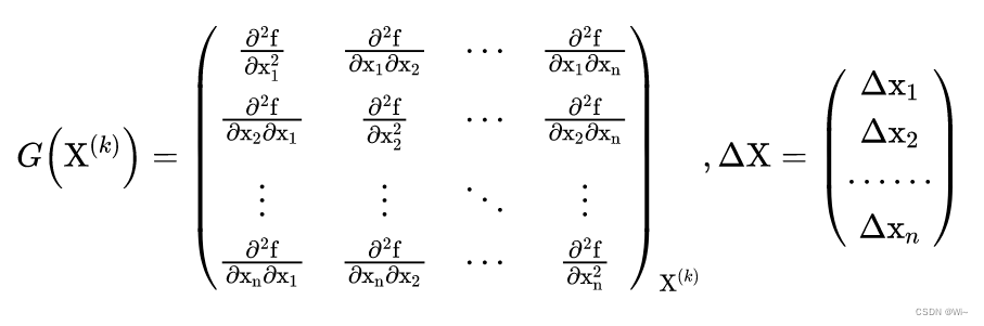
（2）：$G(X^{\left(k\right)})$is$f(x_1,x_2)$ at$X^{}$Hessian matrixat${}^{(}$${}^k$${}^{)}$ . It is given by the function$f(x_1,x_2)$ at$X^{}$The square matrix composed of the second order partial derivatives at${}^{(}$${}^k$${}^{)\; .}$

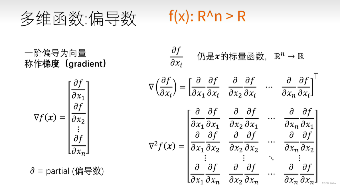
4: Hessian matrix of multivariate functions

1: Multivariate function $f(x_1,x_2,...,x_n)$ at point$x^{}$The Taylor expansion at${}^{(}$${}^k$${}^{)}$
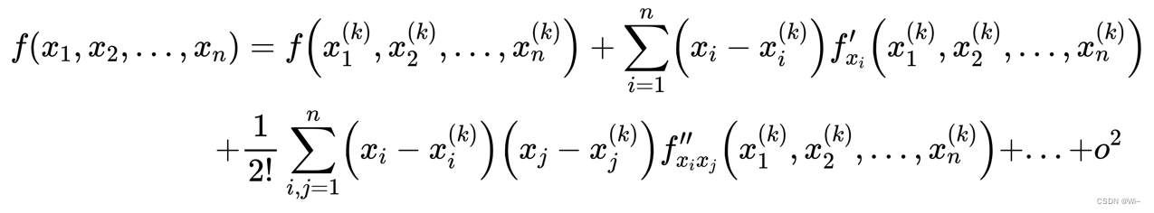is: Write the Taylor (Taylor) expansion in the form of a matrix:
where:

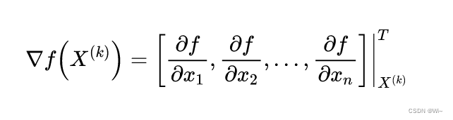
it is$f\left(X\right)$ at$X^{\left(k\right)}$ Gradient at point.
(2):$G(X^{\left(k\right)})$is$f(x_1,x_2,...,x_n)$ at$X^{}$Hessian matrixat${}^{(}$${}^k$${}^{)}$ . It is given by the function$f(x_1,x_2,...,x_n)$ at$X^{\left(k\right)}$ composed of second order partial derivatives$n\ast n$ order square matrix.

2:

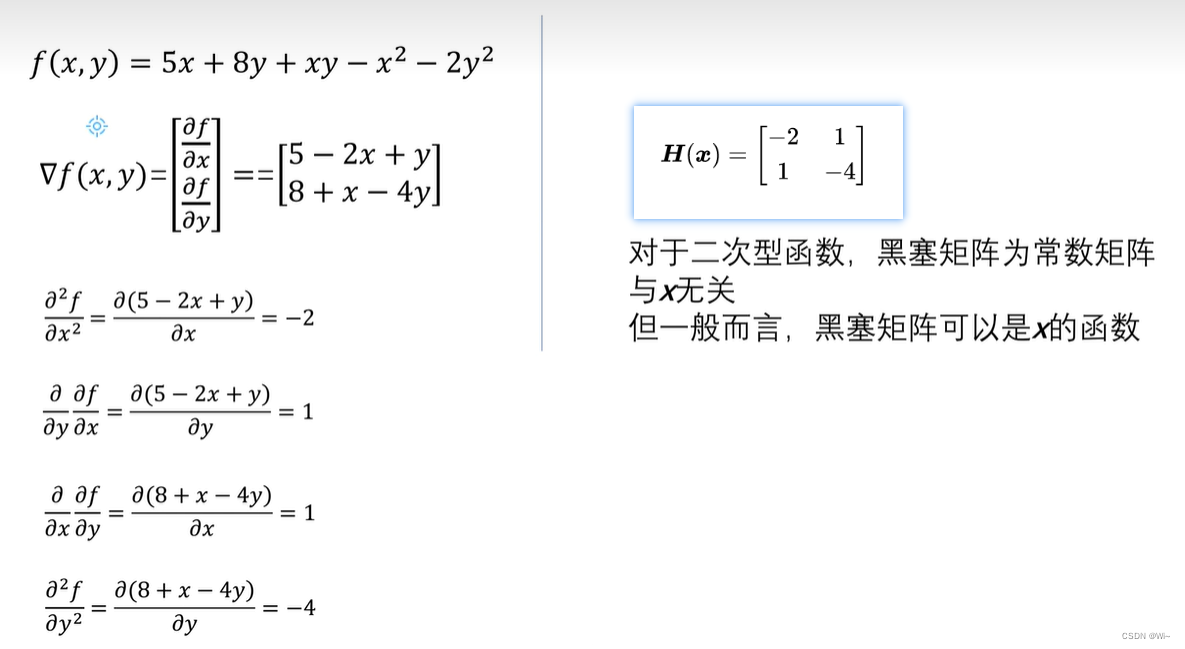
For example:

5: Jacobian matrix of multivariate functions (Jacobian matrix)

1. Overview
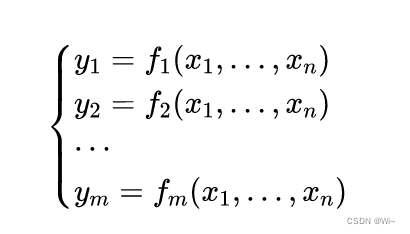
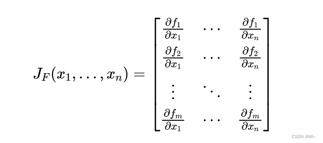
Suppose $f$: $R^n$ → $R^m$ is a function whose input is a vector$x\in R^n$ , the output is the vector$y=f(x)\in R^m$ , and$m\ge n$ is a European style$Convert\; n-$ dimensional space to Euclidean$The\; function\; of\; m-$ dimensional space, this function is determined by$Composed\; of\; m$ real functions:$f_1(x_1,\dots ,x_n)$,…,$f_m(x_1,\dots ,x_n)$ The partial derivatives of these functions (if they exist) can be composed into a$The\; matrix\; of\; m\ast n$ , this is the so-called Jacobian matrix:

Then the Jacobian matrix is ​​an $m\times n$ matrix, usually defined as

2: Example
Let’s look at an actual data fitting process, input:
independent variable: $x=${ $1,2,4,5,8$ }
Dependent variable:$y=${ $3.2939,4.2699,7.1749,9.3008,20.259$ }

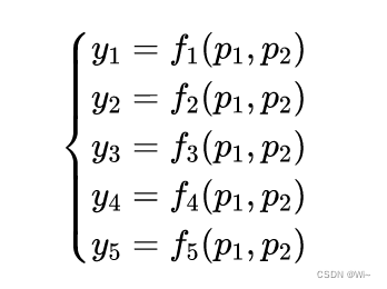
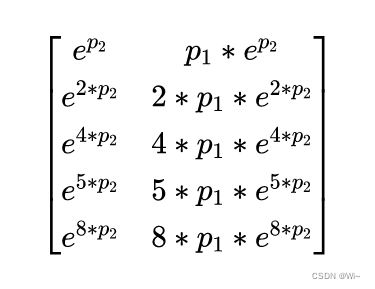
Goal: Use the function $f=p_1\ast e^{p_2\ast x}-y$for fitting, where the independent variable$x$ , dependent variable$y$ , parameter$p_1$and $p_2$, for parameter $p_1$and $p_2$Take the derivative:

$e^{p\ast x}$ versus$p$ is derived:$x\ast e^{p\ast x}$

Jacobian matrix description:

Jacobian矩阵 =

[   exp(p2),     p1*exp(p2)]
[ exp(2*p2), 2*p1*exp(2*p2)]
[ exp(4*p2), 4*p1*exp(4*p2)]
[ exp(5*p2), 5*p1*exp(5*p2)]
[ exp(8*p2), 8*p1*exp(8*p2)]

Right now:

references

Hessian matrix

Hessian and Jacobian matrices

Jacobian Matrix 1

Jacobian Matrix 2
Jacobian Matrix Intuitive Image Understanding