[Literature Reading] Flexible Participation of Devices in Federated Learning

这是张老师的二作文章，可得好好读。

---

Summary

  Traditional federated learning algorithms have strict requirements on the participation rate of devices, which limits the potential coverage of federated learning. This paper extends the current learning paradigm to include devices that may become inactive, compute incomplete updates, and leave or arrive during training. We draw analytical results to illustrate that allowing more flexible device participation affects learning convergence when the data is non-IID.
  We then propose a new federated aggregation scheme that converges even though devices may be inactive or return incomplete updates. We also investigate how the learning process accommodates early departure or late arrival and analyze their impact on convergence.

---

1 Introduction

  Considering that federated learning typically requires thousands of communication rounds to converge, it is difficult in practice to ensure that all devices are available throughout the training process. Additionally, there are often multiple applications running concurrently on user devices, competing for already highly constrained hardware resources. Therefore, there is no guarantee that the device can complete the specified training tasks as expected in each round of training.
  While many methods have been proposed to offload the workload of individual devices, such as weight compression and federated dropout, they cannot completely eliminate the possibility of a device being unable to perform its training duties. Therefore, in large-scale federated learning, many resource-constrained devices must first be excluded from joining federated learning, which limits the potential availability of training datasets and weakens the applicability of federated learning. Furthermore, existing work does not specify how to react when encountering unexpected device behaviors, nor does it analyze the (negative) impact of these behaviors on training progress.
  In this paper, we relax these restrictions and allow devices to follow a more flexible participation model :

• Incompleteness : A device may submit only partially completed work in a round.
• Inactive : Additionally, the device may not complete any updates, or respond to the coordinator at all.
• Early exit : In extreme cases, existing equipment may exit training before completing all training epochs.
• Late Arrivals : In addition to existing equipment, new equipment may join after training has started.

  Our approach to increasing the flexibility of device participation includes the following components, which complement the existing FedAvg algorithm and address the challenges posed by flexible device participation:

• Debiasing of Partial Model Updates
• Fast reboot on device arrival
• Redefining Model Suitability for Device Deviation

---

2 related work

  (Some work on asynchronous training) Asynchronous aggregation in the algorithm can be naturally applied to random inactive devices, but the authors do not analyze how the convergence of their algorithm is affected by inactive or incomplete devices and data heterogeneity.
  (some work that relaxes the device requirements for participation) These works do not show how changes in devices affect the convergence of training, nor do they incorporate user data heterogeneity into the algorithm design.
  Wait for related work research.

---

3 Convergence analysis

3.1 Algorithm description

  Suppose there is $N$ devices, we kkfor each device$k$ defines a local objective function$F_k\left(w\right)$ . in that$w$ is obviously the weight parameter of machine learning,$F_k\left(w\right)$ can be devicekkAverage experience loss over all points over$k\; .$Our global goal is to minimize the following function:

$$F(w)=\sum _{k=1}^N{p}_k{F}_k(w)$$

  where $p^k=\frac{n_k}{n}$，$n_k$is the device kkThe number of data owned by$k$$n={\sum }_{k=1}^N{n}_k$. Order $w^{\ast }$ is the function$F\left(w\right)$ takes the weight parameter of the minimum value. We use$F_k^{\ast }$represents $F_k$minimum value.

  To describe the device kkHow different the data distribution of$k$$C_k=F_k(w^{\ast })-F_k^{\ast }$, at the same time $C={\sum }_{k=1}^N{p}_k{C}_k$.

  Consider discrete time steps $t=0,1,\cdots$ .when$t$ is$When\; the\; multiple\; of\; E$ , the model weights are synchronized. Suppose there are at most$For\; T$ rounds, for each round (eg at$\tau$ round), we perform the following three steps:

1. Synchronization : The server broadcasts the latest weight $w_{\tau E}^{\mathcal{G}}$to all clients. Each client updates its own weight parameter: $w_{\tau E}^k=w_{\tau E}^G$
2. Local training : when $i=0,\cdots ,s_t^k-When\; 1$ , each device has its own loss function$F_k$Transportation SGD calculation: $$w_{\tau E+i+1}^k=w_{\tau E+i}^k-{the}_{}{g}_{\tau E+i}^k$$Here ${the}_{}$is with $\tau$ decaylearning rate,$0\le s_t^k\le E$ represents the number of time steps of local updates done in this round. $g_t^k=\nabla F_k(w_t^k,X_t^k)$ is the device$The\; stochastic\; gradient\; of\; k$ , where$X_t^k$Represents the data of the local mini-batch. We also define ${\bar{g}}_t^k=\nabla F_k(w_t^k)$ means the devicekkThe full batch gradient of$k$${\bar{g}}_t^k={\mathbb{E}}_{X_t^k}[g_t^k]$
3. 码线：电视器砖线梯度可生活在于安全权重parameters：$$\begin{gathered} w_{(\tau +1)E}^{\mathcal{G}}=w_{\tau E}^G+\sum _{k=1}^N{p}_t^k(w_{\tau E+s_t^k}-w_{\tau E}^G) \\ {w}_{(\tau +1)E}^G=w_{\tau E}^G-\sum _{k=1}^N{p}_t^k\sum _{i=0}^{s_t^k}{the}_{}{g}_{\tau E+i}^k \end{gathered}$$If $s_t^k=0$ (that is, device$k$ at the$\tau$ round without any update), then we say device$k$ at the$The\; tau$ round isinactive. If$0<s_t^k<E$ , then we say the device$k$ isincomplete. We will each$s_t^k$As a random variable following any distribution, if $s_t^k$have different distributions, then they are heterogeneous, otherwise they are homogeneous. At the same time, we allow the aggregated weight coefficient $p_t^k$With time steps $\tau$ changes. (Generally$p_t^k$is $s_t^k$The function)

As a special case, traditional FedAvg assumes that all devices complete all $E$ time step training, so$s_t^k\equiv E.$ _ And the aggregation coefficient p τ k ≡ pk p_\tau^k\equiv p^kused by FedAvg participated by all devices$p_t^k\equiv p^k$ , so the right side of the previous formula can be written as:$$w_{(\tau +1)E}^{\mathcal{G}}=\sum _{k=1}^N{p}_t^k{w}_{\tau E}^k$$This is because gradient aggregation is equivalent to directly aggregating model parameters .

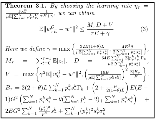
3.2 General convergence bound

  This part proves the following convergence bounds through various assumptions (including Lipschitz gradient, etc.):

3.3 Global Goal Transfer

  This chapter describes the phenomenon that the global loss function is shifted towards the device due to the acceptance of the weights of the specific device. The article has the following theorem:

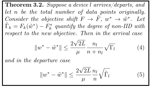
  The article then derives a new convergence bound in the case of global target shifts.