Principles of SQL compilation optimization

Recently, I did some SQL compilation and optimization work on the team's OLAP engine, sorted it out on Yuque, and posted it on the blog by the way. The theory of SQL compilation optimization is not complicated, and it is easier to understand if you only need to master some basics of relational algebra; the more difficult part lies in the reorder algorithm.

basic concept

Relational Algebra Equivalence

Refer to the seventh edition of "Database System Concepts".
The following is the sixth edition


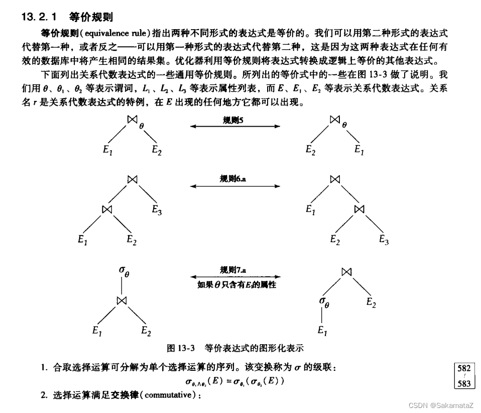
. Note that the commutative laws of natural joins and θ joins cannot be used for outer joins.

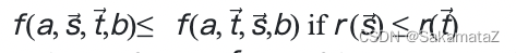
join equivalence rules

https://www.comp.nus.edu.sg/~chancy/sigmod18-reorder.pdf

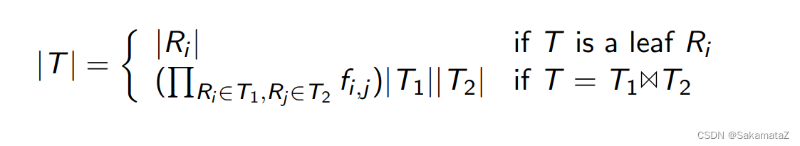
Cardinality

Cardinality represents the number of distinct values

、

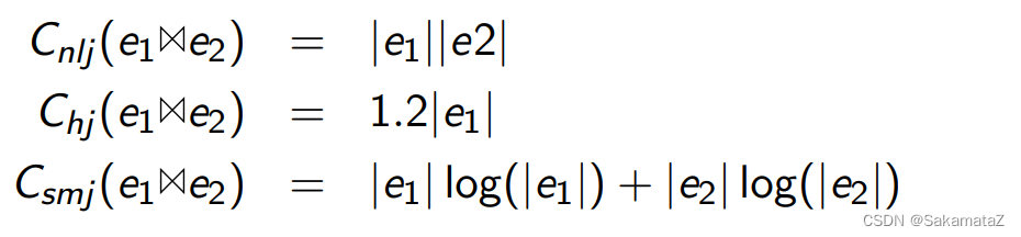
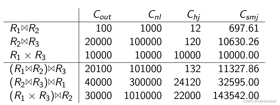
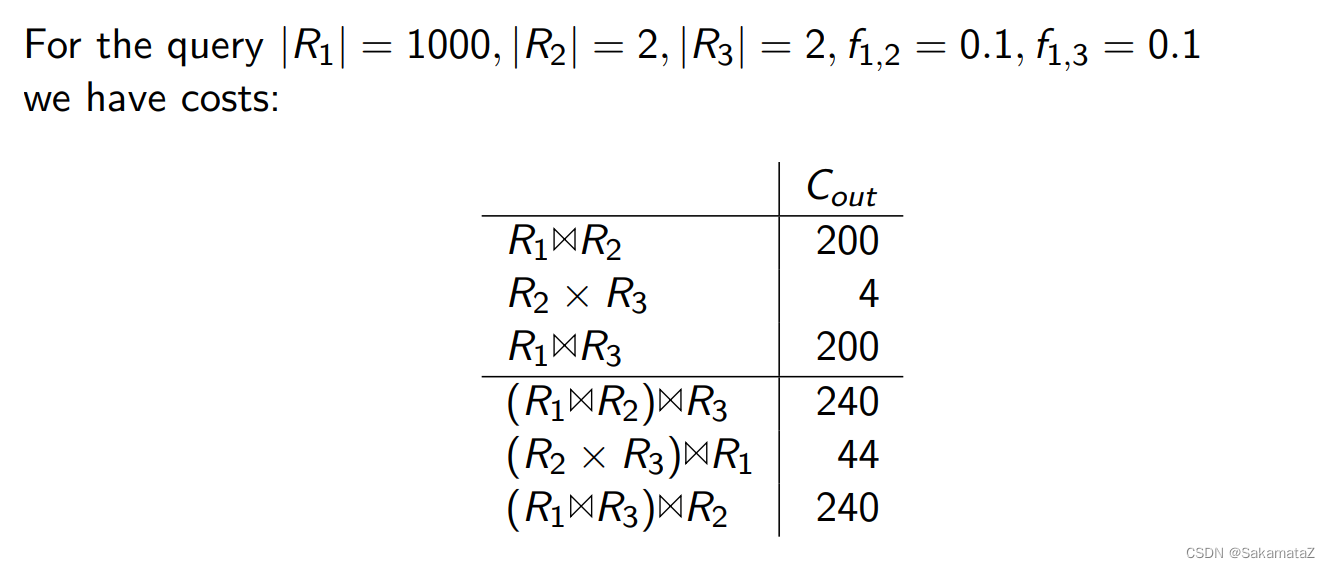
The cost of the join algorithm

From top to bottom, it is nested loop connection, hash connection, sort merge connection

ASI (Adjacent Sequence Interchange)

Classification of query questions

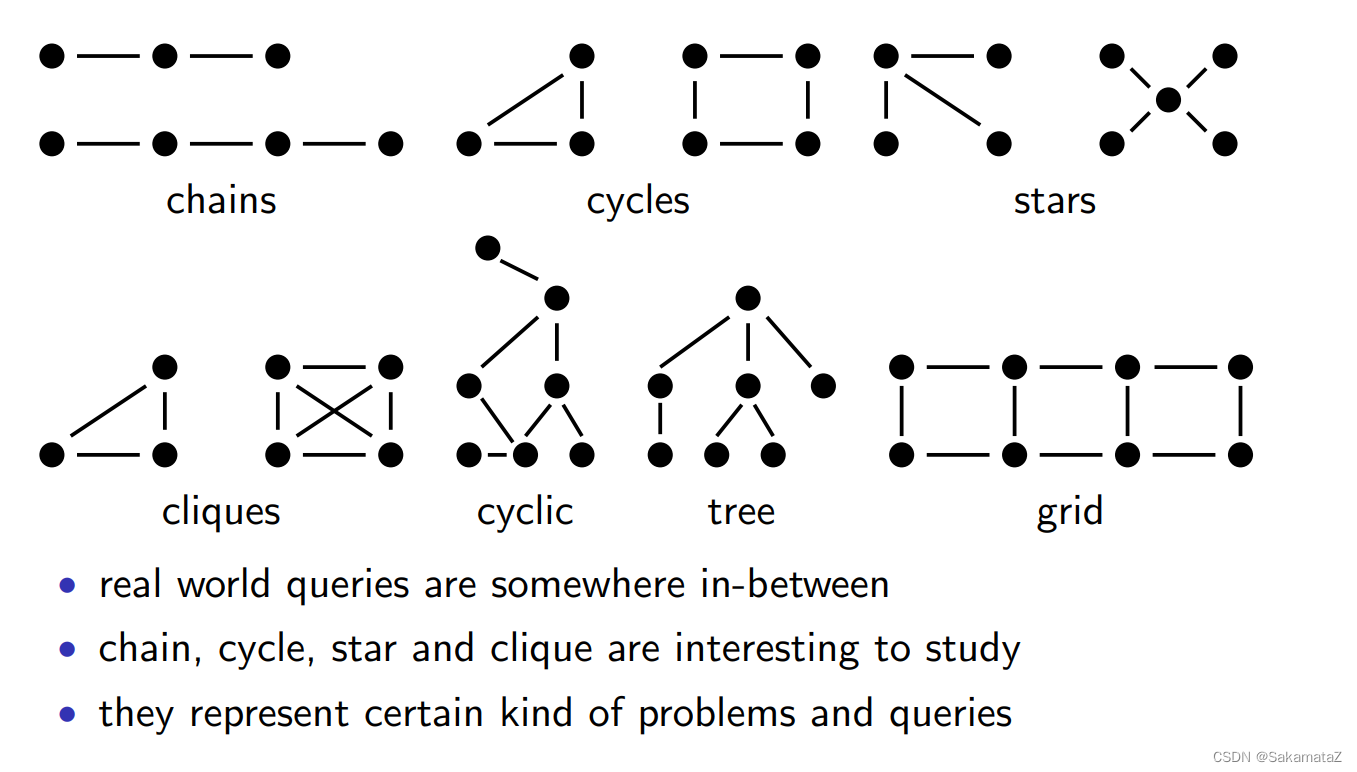
According to the query graph: chain, cycle, star, clique
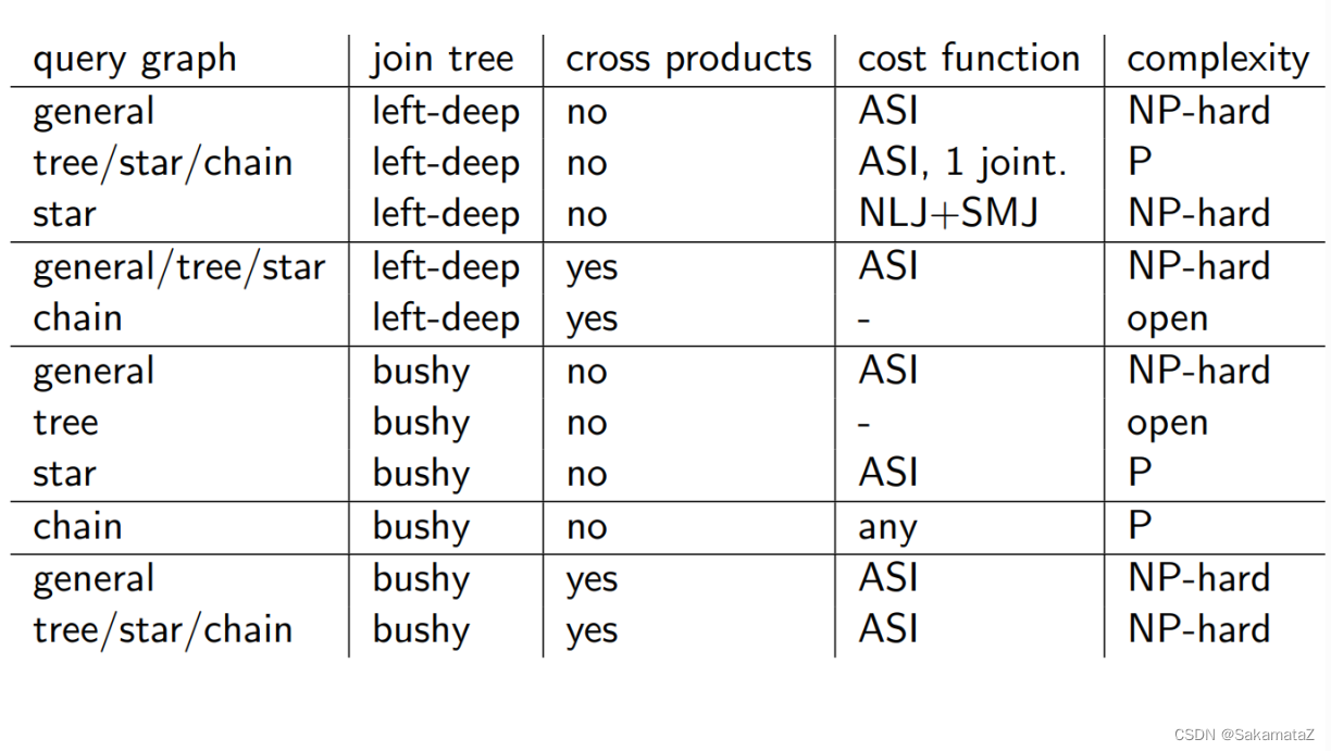
according to the query tree structure: left-deep, zig-zag, bushy tree
according to the join structure: whether there is a cross product
according to the cost function: whether there is an ASI attribute

Possible number of join trees (search space)

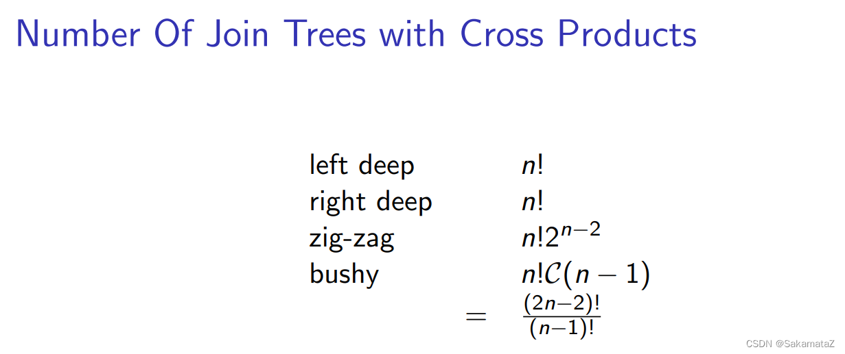
Query graphs, join trees, and problem complexity

Calcite concept

RelNode: plan/subplan
relset: a set of plans equivalent to relational expressions
relsubset: a set of plans equivalent to relational expressions and physical attributes
transformationRule: a set of rules for logical plan changes
converterplan: conversion rules for converting lp to pp
RelOptRule: optimization rules
RelOptNode interface, which represents the expression node
statement that can be operated by the planner: statement
reltrait
RelTraitDef is used to define a class of RelTrait RelTrait
RelTrait is an abstract class that represents the characteristics of query plans. It is used to describe some characteristics of the query plan, and it is a specific instance corresponding to TraitDef.
Convention is a RelTrait used to represent the calling convention of Rel.
rexnode row expression
schema: logical model
Program: a process of parsing and optimizing SQL queries Collection, multiple sub-processes can be combined for parsing and optimization of SQL queries

cascade/volcano

Volcano is a top-down modular prunable SQL optimization model.
Volcano generates two algebraic models: logical and the physical algebras optimize lp and pp respectively (pp mainly selects the execution algorithm).
A volcano optimizer must provide the following parts:
(1) a set of logical operators,
(2) algebraic transformation rules, possibly with condition code,
(3) a set of algorithms and enforcers,
(4) implementation rules, possibly with condition code,
(5) an ADT “cost” with functions for basic arithmetic and comparison,
(6) an ADT “logical properties, ”
(7) an ADT “physical property vector” including comparisons functions (equality and cover),
(8) an applicability function for each algorithm and enforcer,
(9) a cost function for each algorithm and enforcer,
(10) A property function for each operator, algorithm, and enf
volcano uses backward chaining to explore only subqueries and plans that actually participate in larger expressions. This approach avoids searching for irrelevant subqueries and plans, thereby increasing the efficiency of query optimization.

Calcite volcano recursive optimizer implementation

RuleQueue is a priority queue, which contains all currently feasible RuleMatch. In each loop of findBestExpr(), we take out the one with the highest priority and apply it, and then update the queue according to the result of apply...and so on until the termination condition is met.
RuleQueue does not use a large top heap, but only saves the most important nodes.
We imagine that we now have a set of relnodes that match many RuleMatches. How do we decide which match to perform first?
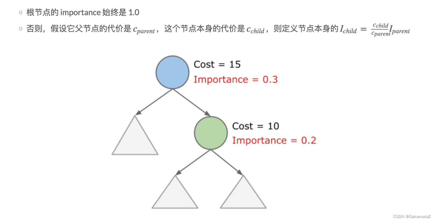
The importance of RuleMatch determines which match is performed first, and the importance of rulematch is defined as the larger of the following two:

1. The importance of the input RelSubset
2. The importance of the output RelSubset
   How to define the importance of the RelSubset? Importance is defined as the larger of the following two:
   ● The real importance of the RelSubset itself
   ● The real importance of any RelSubset that is logically equal (that is, in the same RelSet) is divided by 2. The
   calculation rules for real importance are as follows:
   
   

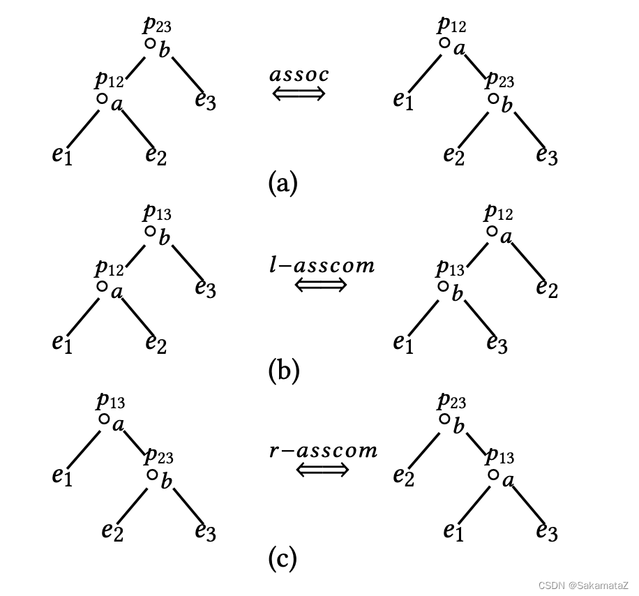
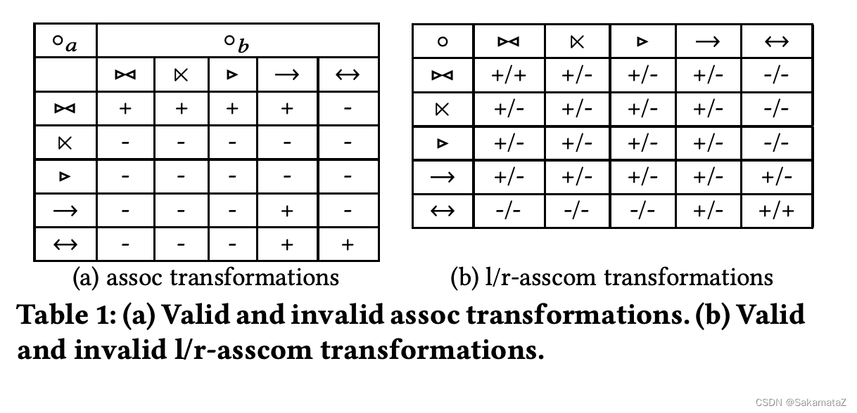
Join reorder

Most of the algorithms are based on connectivity-heuristic, that is, only equl-join is considered

A Dynamic Programming Algorithm Based on Connection Order Optimization

For a collection of n relationships that assume that all connections are natural connections, the complexity of the dynamic programming algorithm is 3^n. The
merge connection can produce ordered results, which may be useful for subsequent sorting (interesting sort order).
At present, we use the connection algorithm of spark, which is temporarily useless.

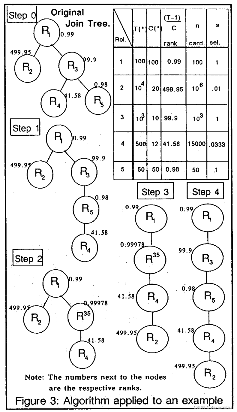
IKKBZ algorithm

left-deep tree and bushy tree
left-deep tree
The right input of the join operator is a concrete relationship, and the right subtree must have a shared predicate with one of the nodes of the left subtree.

The left deep tree is suitable for general scene optimization. The System R optimizer only considers the optimization of the left deep tree, and the time cost is n! , after adding dynamic programming, the optimal connection sequence can be found in n*2^n time.

bushy-tree

Good for multi-way joins and parallel optimization, but complex.
The necessary and sufficient condition for not introducing cross multiplication is that the parent of a given relationship must already be obtained.

BUT

Simply put, it is the principle of equivalent predicate substitution.
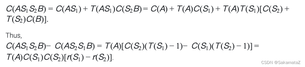
Define the rank function:

Cost function
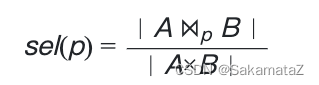
The selectivity of the predicate refers to the ability of the predicate to filter the query results.
For join, the following definitions can be defined:

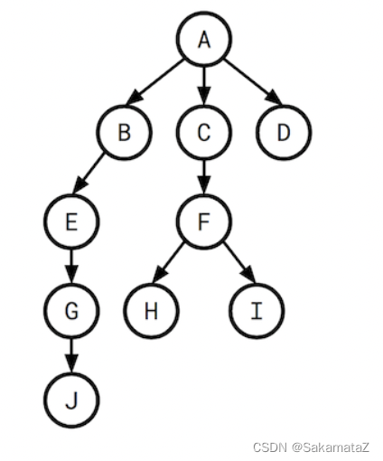
We treat the query graph as a rooted tree, and we say the selectivity of H refers to the selectivity between F and H.
There is the following relationship between the number of rows and selectivity (number of rows * selectivity):

The cost function is defined as follows:

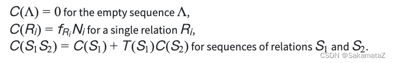
We can define the rank function in terms of the cost function:

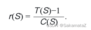
Here is the proof for ASI:

Normalized

Calcite practice

MultiJoinOptimizeBushyRule

The first part is initialized, unusedEdges stores join filter conditions (between two relnodes)

final MultiJoin multiJoinRel = call.rel(0);
    final RexBuilder rexBuilder = multiJoinRel.getCluster().getRexBuilder();
    final RelBuilder relBuilder = call.builder();
    final RelMetadataQuery mq = call.getMetadataQuery();

    final LoptMultiJoin multiJoin = new LoptMultiJoin(multiJoinRel);

    final List<Vertex> vertexes = new ArrayList<>();
    int x = 0;
    for (int i = 0; i < multiJoin.getNumJoinFactors(); i++) {
    
    
      final RelNode rel = multiJoin.getJoinFactor(i);
      double cost = mq.getRowCount(rel);
      vertexes.add(new LeafVertex(i, rel, cost, x));
      x += rel.getRowType().getFieldCount();
    }
    assert x == multiJoin.getNumTotalFields();

    final List<Edge> unusedEdges = new ArrayList<>();
    for (RexNode node : multiJoin.getJoinFilters()) {
    
    
      unusedEdges.add(multiJoin.createEdge(node));
    }

The second step is to select the filter condition with the largest difference in cost (here is the number of rows).
Select a vertex with a smaller number of rows as the majorFactor and the other as the minorFactor

    // Comparator that chooses the best edge. A "good edge" is one that has
    // a large difference in the number of rows on LHS and RHS.
    final Comparator<LoptMultiJoin.Edge> edgeComparator =
        new Comparator<LoptMultiJoin.Edge>() {
    
    
          @Override public int compare(LoptMultiJoin.Edge e0, LoptMultiJoin.Edge e1) {
    
    
            return Double.compare(rowCountDiff(e0), rowCountDiff(e1));
          }

          private double rowCountDiff(LoptMultiJoin.Edge edge) {
    
    
            assert edge.factors.cardinality() == 2 : edge.factors;
            final int factor0 = edge.factors.nextSetBit(0);
            final int factor1 = edge.factors.nextSetBit(factor0 + 1);
            return Math.abs(vertexes.get(factor0).cost
                - vertexes.get(factor1).cost);
          }
        };

    final List<Edge> usedEdges = new ArrayList<>();
    for (;;) {
    
    
      final int edgeOrdinal = chooseBestEdge(unusedEdges, edgeComparator);
      if (pw != null) {
    
    
        trace(vertexes, unusedEdges, usedEdges, edgeOrdinal, pw);
      }
      final int[] factors;
      if (edgeOrdinal == -1) {
    
    
        // No more edges. Are there any un-joined vertexes?
        final Vertex lastVertex = Util.last(vertexes);
        final int z = lastVertex.factors.previousClearBit(lastVertex.id - 1);
        if (z < 0) {
    
    
          break;
        }
        factors = new int[] {
    
    z, lastVertex.id};
      } else {
    
    
        final LoptMultiJoin.Edge bestEdge = unusedEdges.get(edgeOrdinal);

        // For now, assume that the edge is between precisely two factors.
        // 1-factor conditions have probably been pushed down,
        // and 3-or-more-factor conditions are advanced. (TODO:)
        // Therefore, for now, the factors that are merged are exactly the
        // factors on this edge.
        assert bestEdge.factors.cardinality() == 2;
        factors = bestEdge.factors.toArray();
      }
      
      // Determine which factor is to be on the LHS of the join.
      final int majorFactor;
      final int minorFactor;
      if (vertexes.get(factors[0]).cost <= vertexes.get(factors[1]).cost) {
    
    
        majorFactor = factors[0];
        minorFactor = factors[1];
      } else {
    
    
        majorFactor = factors[1];
        minorFactor = factors[0];
      }
      final Vertex majorVertex = vertexes.get(majorFactor);
      final Vertex minorVertex = vertexes.get(minorFactor);

Traversing unusedEdges, adding newFactors, normalizing the previously selected majorVertex and minorVertex and adding vertexes

      // Find the join conditions. All conditions whose factors are now all in
      // the join can now be used.
      final int v = vertexes.size();
      final ImmutableBitSet newFactors =
          majorVertex.factors
              .rebuild()
              .addAll(minorVertex.factors)
              .set(v)
              .build();

      final List<RexNode> conditions = new ArrayList<>();
      final Iterator<LoptMultiJoin.Edge> edgeIterator = unusedEdges.iterator();
      while (edgeIterator.hasNext()) {
    
    
        LoptMultiJoin.Edge edge = edgeIterator.next();
        if (newFactors.contains(edge.factors)) {
    
    
          conditions.add(edge.condition);
          edgeIterator.remove();
          usedEdges.add(edge);
        }
      }
      double cost =
        majorVertex.cost
        * minorVertex.cost
        * RelMdUtil.guessSelectivity(
            RexUtil.composeConjunction(rexBuilder, conditions));
      final Vertex newVertex =
          new JoinVertex(v, majorFactor, minorFactor, newFactors,
              cost, ImmutableList.copyOf(conditions));
      vertexes.add(newVertex);

Selective recalculation after normalization, and then enter the next round

// Re-compute selectivity of edges above the one just chosen.
      // Suppose that we just chose the edge between "product" (10k rows) and
      // "product_class" (10 rows).
      // Both of those vertices are now replaced by a new vertex "P-PC".
      // This vertex has fewer rows (1k rows) -- a fact that is critical to
      // decisions made later. (Hence "greedy" algorithm not "simple".)
      // The adjacent edges are modified.
      final ImmutableBitSet merged =
          ImmutableBitSet.of(minorFactor, majorFactor);
      for (int i = 0; i < unusedEdges.size(); i++) {
    
    
        final LoptMultiJoin.Edge edge = unusedEdges.get(i);
        if (edge.factors.intersects(merged)) {
    
    
          ImmutableBitSet newEdgeFactors =
              edge.factors
                  .rebuild()
                  .removeAll(newFactors)
                  .set(v)
                  .build();
          assert newEdgeFactors.cardinality() == 2;
          final LoptMultiJoin.Edge newEdge =
              new LoptMultiJoin.Edge(edge.condition, newEdgeFactors,
                  edge.columns);
          unusedEdges.set(i, newEdge);
        }
      }

In the last paragraph, create a relnode node according to the new vertexes order

// We have a winner!
List<Pair<RelNode, TargetMapping>> relNodes = new ArrayList<>();
for (Vertex vertex : vertexes) {
    
    
  if (vertex instanceof LeafVertex) {
    
    
    LeafVertex leafVertex = (LeafVertex) vertex;
    final Mappings.TargetMapping mapping =
        Mappings.offsetSource(
            Mappings.createIdentity(
                leafVertex.rel.getRowType().getFieldCount()),
            leafVertex.fieldOffset,
            multiJoin.getNumTotalFields());
    relNodes.add(Pair.of(leafVertex.rel, mapping));
  } else {
    
    
    JoinVertex joinVertex = (JoinVertex) vertex;
    final Pair<RelNode, Mappings.TargetMapping> leftPair =
        relNodes.get(joinVertex.leftFactor);
    RelNode left = leftPair.left;
    final Mappings.TargetMapping leftMapping = leftPair.right;
    final Pair<RelNode, Mappings.TargetMapping> rightPair =
        relNodes.get(joinVertex.rightFactor);
    RelNode right = rightPair.left;
    final Mappings.TargetMapping rightMapping = rightPair.right;
    final Mappings.TargetMapping mapping =
        Mappings.merge(leftMapping,
            Mappings.offsetTarget(rightMapping,
                left.getRowType().getFieldCount()));
    if (pw != null) {
    
    
      pw.println("left: " + leftMapping);
      pw.println("right: " + rightMapping);
      pw.println("combined: " + mapping);
      pw.println();
    }
    final RexVisitor<RexNode> shuttle =
        new RexPermuteInputsShuttle(mapping, left, right);
    final RexNode condition =
        RexUtil.composeConjunction(rexBuilder, joinVertex.conditions);

    final RelNode join = relBuilder.push(left)
        .push(right)
        .join(JoinRelType.INNER, condition.accept(shuttle))
        .build();
    relNodes.add(Pair.of(join, mapping));
  }
  if (pw != null) {
    
    
    pw.println(Util.last(relNodes));
  }

Join Algorithm Selection

Correlated subquery optimization

We call the operator connecting the external query and subquery CorrelatedJoin (also known as lateral join, dependent join, apply operator, etc. Its left subtree is called external query (input), and its right subtree is called For the subquery (subquery).

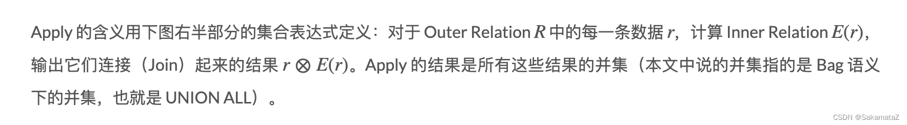
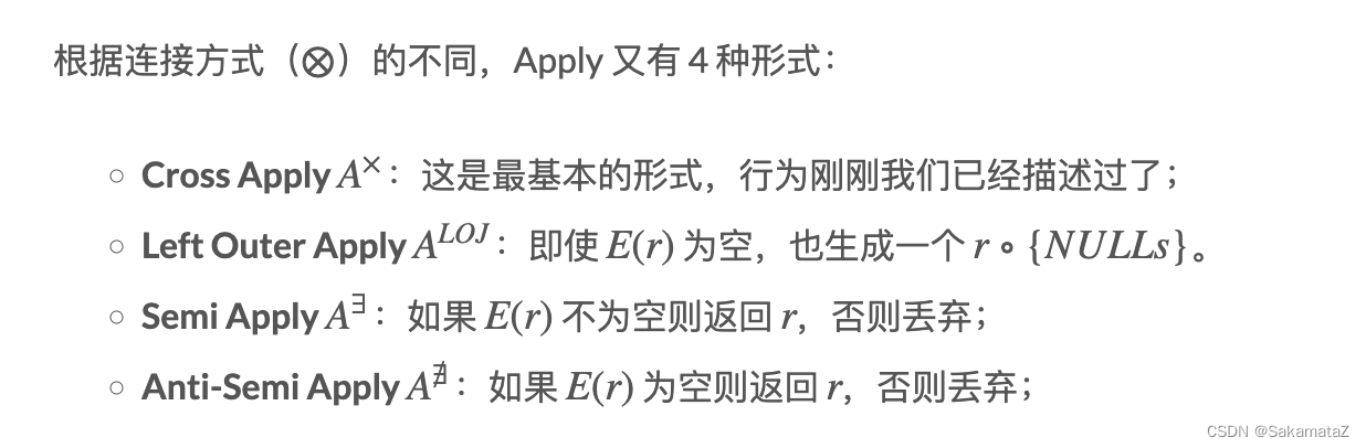
Note: bag semantics, allowing elements to appear repeatedly, are orthogonal to set semantics

Why eliminate correlated subqueries?

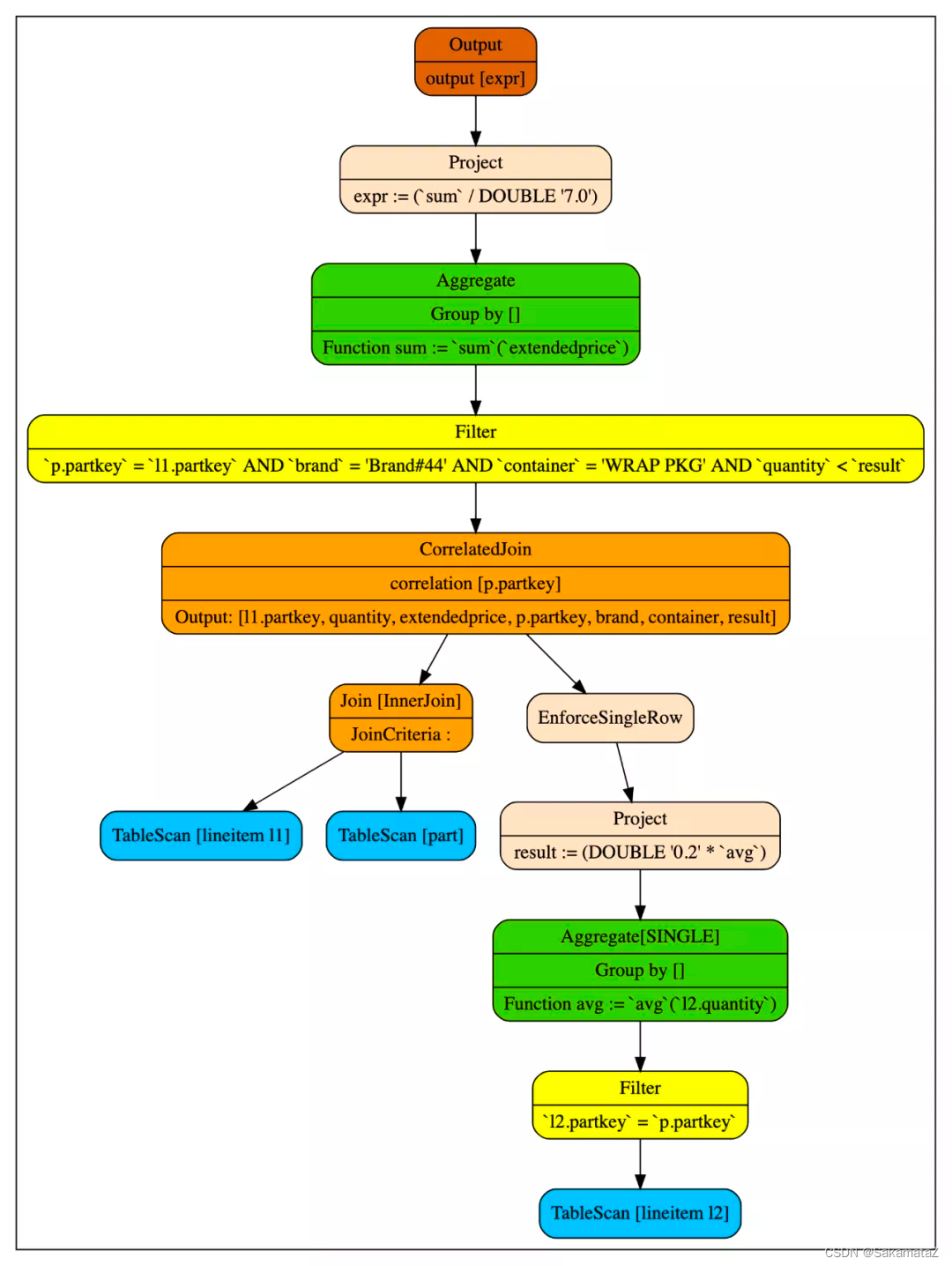
The CorrelatedJoin operator breaks the previous top-down execution mode of the logic tree. Ordinary logical trees are executed from the leaf node to the root node, but the right subtree of CorreltedJoin will be repeatedly executed by the value of the row brought into the left subtree.

Basic Elimination Rules

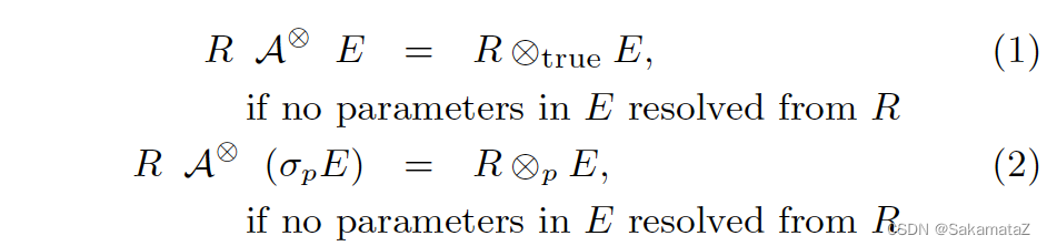
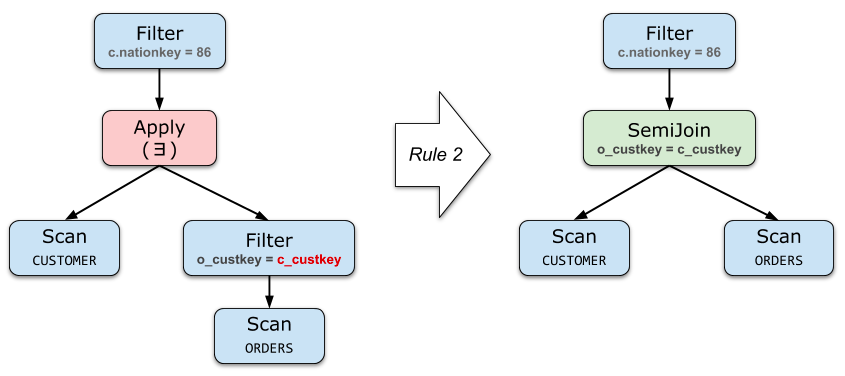
If the right side of Apply does not contain parameters from the left (or only contains filter parameters), then it is equivalent to direct Join

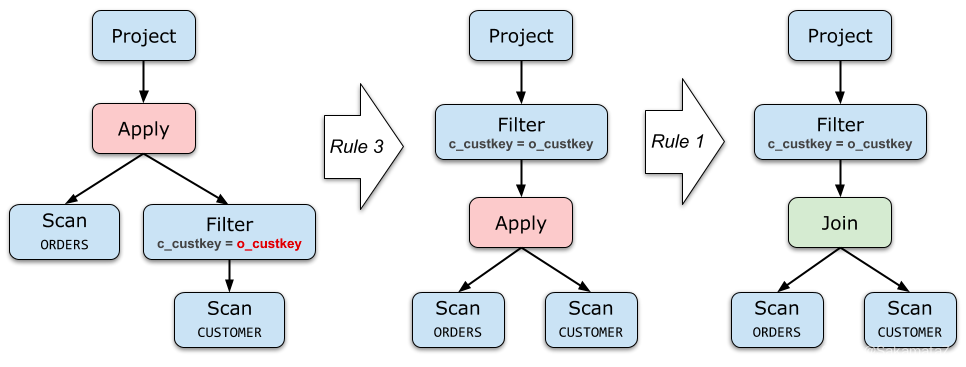
Project and filter de-association

Push down Apply as much as possible, and lift up the operator below Apply.

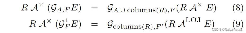
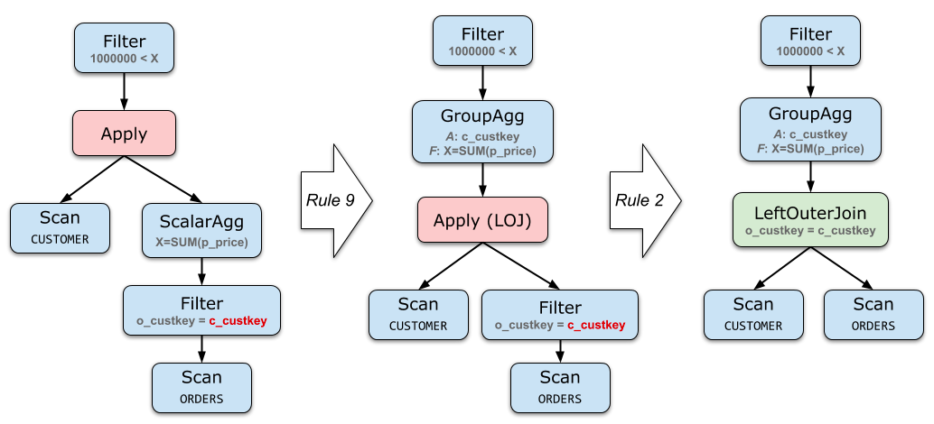
Aggregate de-association

SELECT c_custkey
FROM CUSTOMER
WHERE 1000000 < (
    SELECT SUM(o_totalprice)
    FROM ORDERS
    WHERE o_custkey = c_custkey
)
// 等价于
select sum(p_price) > 1000000 from CUSTOMER.o_custkey left join ORDERS.c_custkey 
on CUSTOMER.o_custkey = ORDERS.c_custkey group by ORDERS.c_custkey

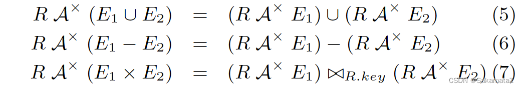
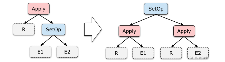
Disassociation of set operations

This set of rules rarely comes in handy. Under TPC-H's Schema, it is even difficult to write a meaningful subquery with Union All.