1. Description
In machine learning (ML), some of the most important linear algebra concepts are singular value decomposition (SVD) and principal component analysis (PCA). With all the raw data collected, how do we discover structure? For example, with interest rates for the past 6 days, can we understand its composition to spot trends?
For high-dimensional raw data, this becomes more difficult. It's like finding a needle in a haystack. SVD allows us to extract and unpack information. In this article, we will introduce SVD and PCA in detail. We assume that you have basic knowledge of linear algebra, including rank and eigenvectors . If you are having trouble reading this article, I recommend that you refresh these concepts first. At the end of the article, we will answer some questions from the interest rate example above. This article also contains optional sections. Feel free to skip it depending on your interest level.
2. Misunderstanding (optional for beginners)
I realize some common questions non-beginners might ask. Let me start by talking about the elephant in the room. Does the PCA size decrease? PCA reduces dimensions, but it's much more than that. I like the wiki's description (but if you don't know PCA, it's just gibberish):
Principal Component Analysis (PCA) is a statistical procedure that uses an orthogonal transformation to convert a set of observations of potentially correlated variables (with various values for each entity) into a set of linearly uncorrelated variable values, called main ingredient.
From a simplistic perspective, PCA linearly transforms the data into new attributes that are uncorrelated with each other. For ML, positioning PCA as feature extraction may allow us to explore its potential better than dimensionality reduction.
What is the difference between SVD and PCA? SVD gives you the whole nine yards of diagonalizing matrices into special matrices that are easy to manipulate and analyze. It lays the foundation for untangling data into independent components. PCA skips less important components. Clearly, we can use SVD to find PCA by truncating less important basis vectors in the original SVD matrix.
Fourth, matrix diagonalization
In the paper on eigenvalues and eigenvectors , we described a method for decomposing an n × n square matrix A into
![]()
For example

If A is a square matrix with n linearly independent eigenvectors , then the matrix can be diagonalized. Now, it's time to develop solutions for all matrices using SVD.
5. Singular vectors and singular values
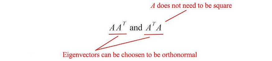
The matrices AAT and ATA are very special in linear algebra. Consider any m×n matrix A , we can multiply it with AT to form AAT and ATA , respectively . These matrices are
- symmetry
- square
- is at least positive semidefinite (eigenvalues are zero or positive),
- Both matrices have the same positive eigenvalues, and
- Both have the same rank r as A.
Also, the covariance matrix we often use in ML takes this form. Since they are symmetric, we can choose their eigenvectors to be orthonormal (perpendicular to each other with unit length) - a fundamental property of symmetric matrices .
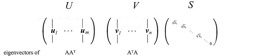
Let us introduce some frequently used terms in SVD. We name the eigenvectors of AAT as ui and ATA as vi , and call these set of eigenvectors u and v as the singular vectors of A. Both matrices have the same positive eigenvalues. The square roots of these eigenvalues are called singular values .
Not much explanation so far, but let's put everything together first and explain next. We concatenate the vectors ui to U and vi to V to form an orthogonal matrix.

Since these vectors are orthogonal, it is easy to show that U and V obey

6. SVD
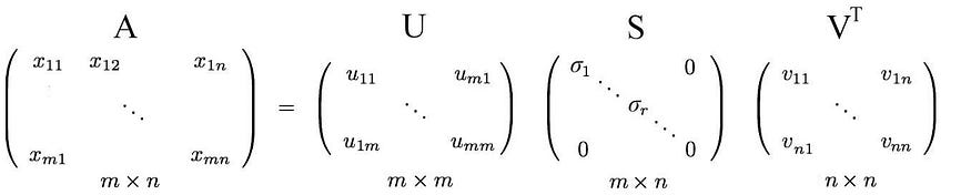
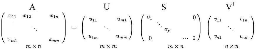
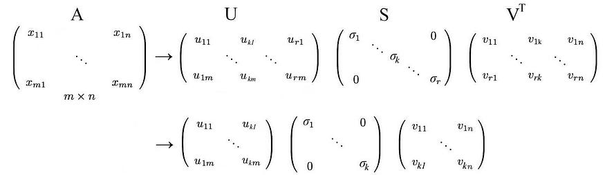
Let's start with the hard part first. SVD states that any matrix A can be decomposed as:

where U and V are orthogonal matrices, and the orthogonal eigenvectors are selected from AAT and ATA , respectively . S is a diagonal matrix with r elements equal to the roots of the positive eigenvalues of AAT or AT A (both matrices have the same positive eigenvalues anyway). The diagonal elements consist of singular values.

i.e. an m× n matrix can be factorized as:

We can arrange the eigenvectors in different orders to produce U and V. To normalize the solution, we order the eigenvectors such that vectors with higher eigenvalues are preferred over vectors with smaller eigenvalues.

In contrast to eigendecomposition, SVD works for non-square matrices. U and V are invertible for any matrix in SVD, they are orthogonal matrices which we like. If there is no evidence, we also told you that singular values are more stable than eigenvalues.
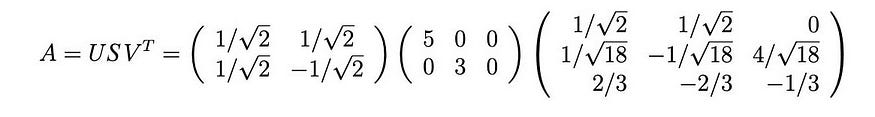
Example ( example source )
Before going too far, let's demonstrate it with a simple example. This will make things very easy to understand.

We calculate:

These matrices are at least positive semidefinite (all eigenvalues are positive or zero). As shown, they have the same positive eigenvalues (25 and 9). The figure below also shows their corresponding eigenvectors.
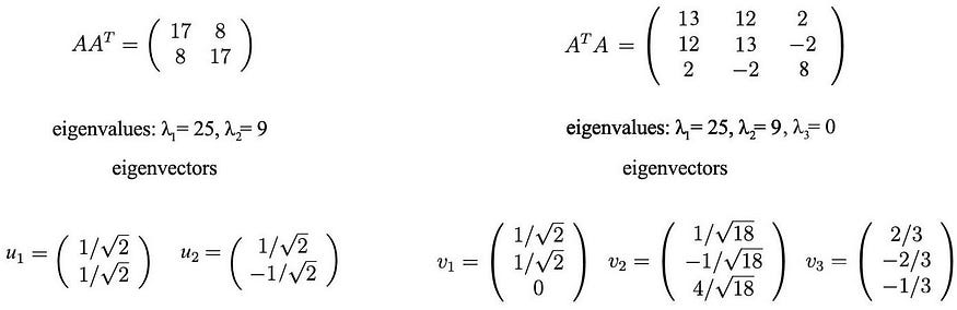
The singular values are the square roots of the positive eigenvalues, 5 and 3. Therefore, the SVD composition is
7. Proof (optional)
To demonstrate SVD, we wish to solve for U, S and V with the following formulas :

We have 3 unknowns. Hopefully we can solve them with the 3 equations above. The transpose of A is

understanding

We calculate ATA ,

The last equation is equivalent to the definition of the eigenvectors of the matrix ( ATA ) . We just put all the eigenvectors in one matrix.
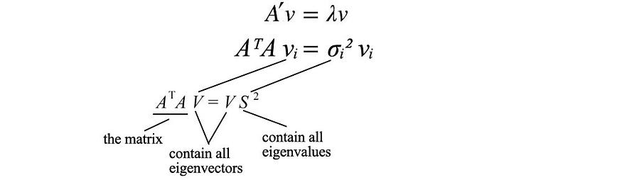
with VS² equal to

V holds all eigenvectors vi of ATA , and S holds the square root of all eigenvalues of ATA . We can repeat the same process for AAT and return a similar equation.

Now, we only need to solve for U, V and S

and prove the theorem.
8. Review
The following is a review of SVD.

where
9. Re-enactment of SVD
Since the matrix V is orthogonal, VTV is equal to I. We can rewrite the SVD equation as:

This equation establishes an important relationship between UI and VI .
recall

apply AV=US ,
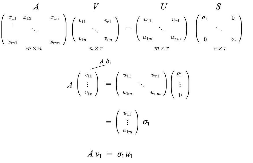
This can be summarized as

Equivalent to

and

The SVD decomposition can be identified as a series of outer products of ui and vi .

This formulation of SVD is key to understanding the components of A. It provides an important way to decompose m × n arrays of entangled data into r components. Since ui and vi are unit vectors, we can even ignore terms with very small singular values σi ( σiuiviT ). (We'll come back to this question later.
Let's start by reusing the previous example and showing how it works.
The above matrix A can be decomposed into

10. Column Space, Row Space, Left Space and Empty Space (optional - for advanced users)
Next, we'll look at what U & V consist of. Suppose A is an m × n matrix of rank r . ATA will be an nxn symmetric matrix. All symmetric matrices have a choice of n orthogonal eigenvectors vj . Since Avi = σiui and vj are orthogonal eigenvectors of ATA , we can calculate the value of ui T uj as

It is equal to zero. That is, UI and uj are orthogonal to each other. As mentioned earlier, they are also the eigenvectors of AAT .
From Avi = σui , we can realize that ui is the column vector of A.

Since A has rank r, we can choose these r ui vectors as orthogonal vectors. So what are the remaining mr-orthogonal eigenvectors of AAT ? Since the left null space of A is orthogonal to the column space, it is natural to choose them as the remaining eigenvectors. (The zero point N ( AT) on the left is the spatial span of x in ATx=0 . Similar parameters apply to the eigenvectors of ATA . Therefore
Returning to the previous SVD equation, from
We just put the eigenvectors back into the left and null spaces.
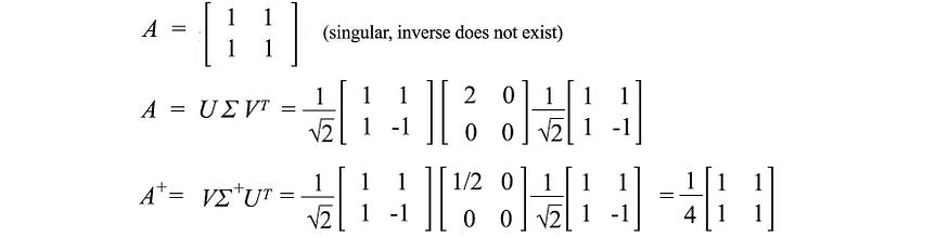
11. Moore-Penrose Pseudoinverse
For a system of linear equations, we can compute the inverse of the square matrix A to solve for x .

But not all matrices are invertible. Also, in ML, finding an exact solution is unlikely in the presence of noise in the data. Our goal is to find the model that best fits the data. To find the most suitable solution, we compute a pseudoinverse
![]()
This minimizes the least squares error below.
![]()
The solution for x can be estimated as,

In a linear regression problem, x is our linear model, A contains the training data, and b contains the corresponding labels. We can solve x by


Below is an example.
12. Variance and covariance
In ML, we recognize patterns and relationships. How do we identify correlations of attributes in data? Let's start the discussion with an example. We sample the height and weight of 12 people and calculate their average. We zero it out by subtracting the original value from its mean. For example, matrix A below holds the adjusted zero center height and weight.

When we plot the data points, we can realize that height and weight are positively correlated. But how do we quantify this relationship?
First, how is real estate different? We probably start learning the difference in high school. Let us introduce its cousin. The sample variance is defined as:

Note that it divides by n-1 instead of n in the variance . With a finite sample size, the sample mean is biased and sample dependent. The average squared distance from this mean will be smaller than the average squared distance from the general population. Dividing the sample covariance S ² by n-1 compensates for small values and can be shown to be an unbiased estimator of the variance σ ² . (The proof is not very important, so I simply provide a link to the proof here .
Thirteen, covariance matrix
Variance measures how a variable varies among itself, while covariance varies between two variables ( a and b ).

We can store all these possible combinations of covariances in a matrix called the covariance matrix Σ.

We can rewrite it in simple matrix form.

The diagonal elements hold the variance of each variable (such as height), and the off-diagonal elements hold the covariance between two variables. Now let's calculate the sample covariance.


A positive sample covariance indicates that weight and height are positively related. Negative if they are negatively correlated, zero if they are independent.
Covariance Matrix and SVD
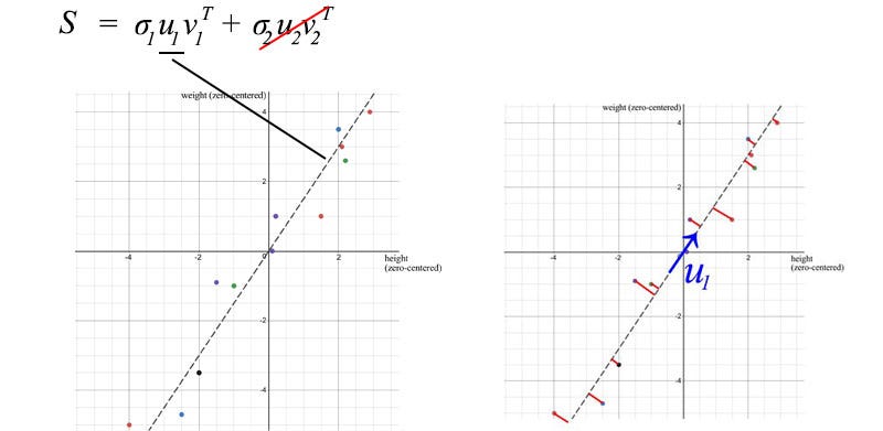
We can use SVD to decompose the sample covariance matrix. Since σ₂ is relatively small compared to σ₁ , we can even ignore the σ₂ term . When we train an ML model, we can perform linear regression on weight and height to form a new attribute, rather than treating them as two separate and related attributes (entangled data often makes model training more difficult).

U₁ has an important importance. It is the main component of S.
The sample covariance matrix in the context of SVD has several properties:
- The total variance of the data is equal to the trace of the sample covariance matrix S, which is equal to the sum of squares of the singular values of S. With this, we can calculate the ratio of variance lost if we remove the smaller σi terms . This reflects how much information would be lost if we eliminated them.
![]()
- The first eigenvector u₁ of S points in the most important direction of the data. In our example, it quantifies the typical ratio between weight and height.
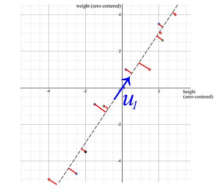
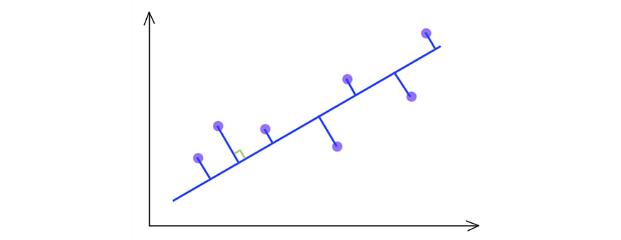
vertical least squares
- The error is calculated as the sum of the vertical squared distances from the sample point to u₁ , which is the minimum value when using SVD.
property
The covariance matrix is not only symmetric, but also positive semidefinite. Since the variance is positive or zero, uTVu below is always greater than or equal to zero. By energy test, V is positive semidefinite.

therefore
![]()
Usually, after some linear transformation of A , we want to know the covariance of the transformed data. This can be calculated using the transformation matrix A and the covariance of the original data.

correlation matrix
The correlation matrix is a scaled version of the covariance matrix. The correlation matrix standardizes (scales) the variables to have a standard deviation of 1.
If the variables are on very different scales, a correlation matrix will be used. Bad scaling can harm ML algorithms like gradient descent.
14. Visualization
So far we have many equations. Let's visualize SVD in action and develop insights step by step. SVD decomposes matrix A into USVT. Applying A to a vector x ( Ax ) can be visualized as performing a rotation ( VT ), scaling ( S ) and another rotation ( U ) on x .

As shown above, the eigenvector vi of V is transformed into:

or in full matrix form

demonstrate that r = m < n
15. Insights from SVD
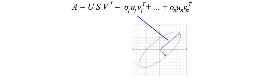
As mentioned earlier, SVD can be expressed as

Since ui and vi have unit length, the most important factor determining the importance of each term is the singular value σi . We purposely sort σi in descending order . If the eigenvalues become too small, we can ignore the remaining terms (+ σiuiviT + ... ).

This formulaicity has some interesting implications. For example, we have a matrix that contains the return of stock returns traded by different investors.
As fund managers, what information can we learn from this? Finding patterns and structures will be the first step. Perhaps, we can identify the highest yielding stocks and investor combinations. SVD decomposes n × n matrices into r components, and the singular value σi indicates its significance. Think of this as a way to extract entanglement and correlation properties into fewer principal directions with no correlations.
![]()
If the data are highly correlated, we should expect many σi values to be small and negligible.
In our previous example, weight and height were highly correlated. If we have a matrix with weights and heights of 1000 people, the first component in the SVD decomposition will dominate. The u₁ vector does show the ratio between weight and height among the 1000 people we discussed earlier.
16. Principal Component Analysis
Technically speaking, SVD extracts data separately in the direction of greatest variance. PCA is a linear model that maps m- dimensional input features to k-dimensional latent factors ( k principal components). If we ignore the less important terms, we remove less caring components but keep the main directions with the highest variance (maximum information).

Consider the 3D data points shown below as blue dots. It can be easily approximated with a plane.
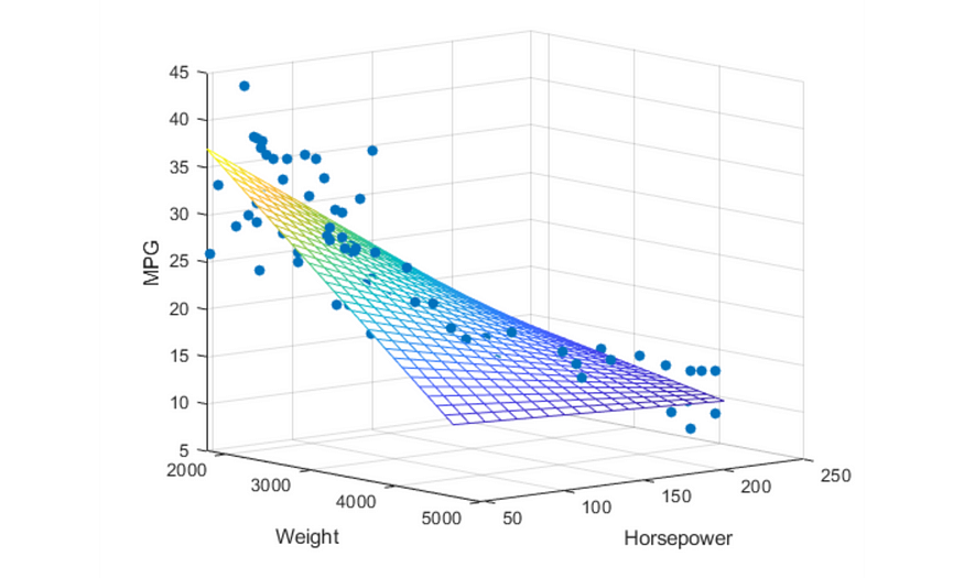
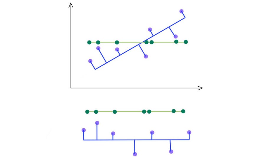
You may quickly realize that we can use SVD to find the matrix W . Consider the following data points lying on two-dimensional space.
SVD chooses the projection that maximizes the variance of its output. Therefore, if the variance is higher, PCA will choose the blue line instead of the green line.
As indicated below, we keep the eigenvectors that have the top kth highest singular value.
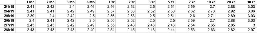
interest rate
Let's illustrate this concept in more depth by tracing interest rate data from the U.S. Treasury Department. Basis points for 9 different rates (from 3 months, 6 months, ... to 20 years) collected over 6 consecutive business days, A stores the difference from the previous date. During this time, the elements of A have also had their averages subtracted. i.e. it is zero-centered (across its rows).

The sample covariance matrix is equal to S = AAT/(5–1).
Now we have the covariance matrix S that we want to decompose . SVD decomposes into

From the SVD decomposition, we realize that we can focus on the first three principal components.

As shown, the first principal component is related to the weighted average of the daily changes across all maturities. The second principal component adjusts for daily changes that are sensitive to bond maturity. (A third principal component might be curvature - the second derivative.
We know all too well the relationship between interest rate changes and maturity dates in our daily lives. Therefore, the principal components reaffirm our view on the behavior of interest rates. However, when we see unfamiliar raw data, PCA is very helpful in extracting the main components of the data to find the underlying information structure. This might answer some questions about how to find the needle in the haystack.
Seventeen, skills
Scales features before performing SVD.

For example, if we want to retain 99% of the variance, we can choose k like this
