Linear regression practice 1: Predicting Boston housing prices

The boston house price data set includes 506 samples, each sample includes 13 characteristic variables and the average house price in the area. The house price is obviously related to multiple characteristic variables. For the linear regression model, first select a linear regression with multiple features to establish a linear equation , observe the quality of the model prediction, and then choose multiple linear regression for house price prediction.

Simple Linear Regression: When the regression model contains one dependent variable and one independent variable.
Polynomial regression: When there is only one independent variable, but also contains the power of the variable (X2, X3), it is called polynomial regression.
Multiple Linear Regression: When there is more than one independent variable.

 1. Load the dataset

1. Guide package

import matplotlib.pyplot as plt
import numpy as np
import pandas as pd
import xgboost as xgb
from sklearn import datasets
from sklearn.model_selection import train_test_split, GridSearchCV
from sklearn.metrics import mean_squared_error

2. Read in data and display

boston = datasets.load_boston()
data = pd.DataFrame(boston.data)
data.columns = boston.feature_names
data['price'] = boston.target
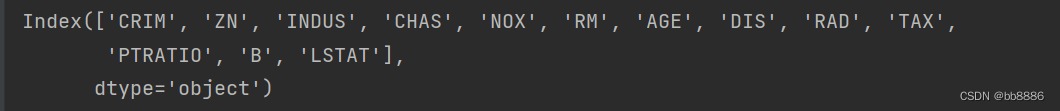
print(data.columns)
print(data.head())

Features (13): 

 First few lines of data: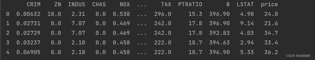

3. Split features and labels

y = data.pop('price')

2. Data set processing

1. Check the null value

print(data.isnull().sum())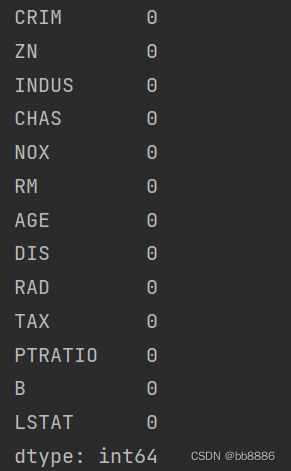

2. Check the data size

print(data.shape)

3. View data description information

print(data.describe())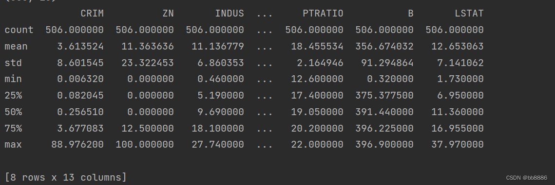

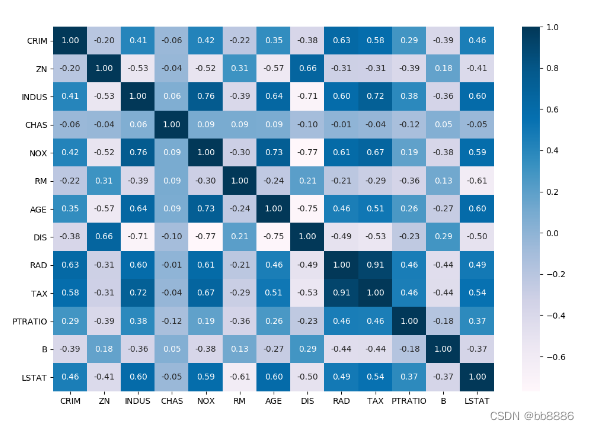
4. View the correlation of each feature

import seaborn as sns
plt.figure(figsize=(12, 8))
sns.heatmap(data.corr(), annot=True, fmt='.2f', cmap='PuBu')
plt.show()

5. Draw a scatter diagram of each feature and house price

data_xTitle = ['CRIM','ZN','INDUS','CHAS','NOX','RM','AGE','DIS','RAD','TAX','PTRATIO','B', 'LSTAT']
plt.figure(figsize=[20,18])
fig, a = plt.subplots(5, 3)
m = 0
for i in range(0, 5):
    if i == 4:
        a[i][0].scatter(data[str(data_xTitle[m])], y, s=30, edgecolor='white')
        a[i][0].set_title(str(data_xTitle[m]))
    else:
        for j in range(0, 3):
            a[i][j].scatter(data[str(data_xTitle[m])], y, s=30, edgecolor='white')
            a[i][j].set_title(str(data_xTitle[m]))
            m = m + 1
plt.show()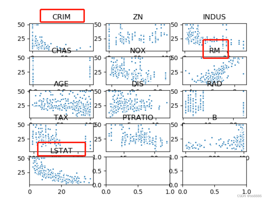

It can be seen from the above figure that the three eigenvalues ​​of 'RM', 'LSTAT', and 'CRIM' have a certain correlation with housing prices, so these three characteristics are selected as eigenvalues, and the remaining irrelevant eigenvalues ​​are removed.

new_boston_df = data[['LSTAT', 'CRIM', 'RM']]
print(new_boston_df.describe())
new_boston_df = np.array(new_boston_df)
data = np.array(data)
y = np.array(y)

 6. Divide the dataset

x_train, x_test, y_train, y_test = train_test_split(data, y, test_size=0.2, random_state=14)

3. Establish a linear model

1. Establish a linear regression model

We use the features before selection (13) and features after selection (3) to model and draw the fitting curve.

data_list = [data, new_boston_df]


for index, data in enumerate(data_list):
    x_train, x_test, y_train, y_test = train_test_split(data, y, test_size=0.2, random_state=14)

    # 线性回归
    lr_reg = linear_model.LinearRegression()
    lr_reg.fit(x_train, y_train)
    print("线性回归的系数：w = {}, b = {}".format(lr_reg.coef_, lr_reg.intercept_))
    pred = lr_reg.predict(x_test)
    train_pred = lr_reg.predict(x_train)
    # 计算MSE
    test_MSE =mean_squared_error(pred, y_test)
    train_MSE = mean_squared_error(train_pred, y_train)
    # 计算MAE
    test_MAE = mean_absolute_error(y_test, pred)
    train_MAE = mean_absolute_error(y_train, train_pred)
    score = lr_reg.score(x_test, y_test)
    # 预测值与真实值的可视化
    y_test = tuple(y_test)
    test = []
    pre = []
    for i in np.argsort(pred):
        test.append(y_test[i])
        pre.append(pred[i])
    plt.plot(test, label='true')
    plt.plot(pre, label='predict')
    if index == 0:
        plt.title('all_feature,ACC:{:.2f}%,MSE:{:.2f},MAE:{:.2f}'.format(score*100, test_MSE, test_MAE))
    else:
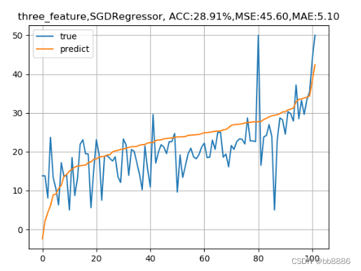
        plt.title('three_feature,ACC:{:.2f}%,MSE:{:.2f},MAE:{:.2f}'.format(score*100, test_MSE, test_MAE))
    plt.legend()
    plt.grid()
    plt.show()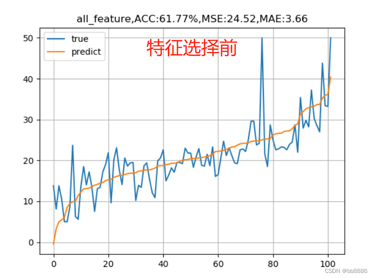

 We found that the accuracy rate before feature selection is higher than that after feature selection, and the mean square error is also smaller than that after feature selection. Why? Below we use the features before and after feature selection, respectively, and use SDG, ridge regression and Lasso regression to observe the model results.

2、SDG

3. Ridge regression

4. Lasso regression

On the basis of the above, we added two more linear models, SGD linear model and linear regression + L2 regularization .

1. Linear regression for solving normal equations is suitable for data with not too many features and not particularly complex .

2. SGD linear regression, stochastic gradient descent linear regression, sgd is suitable for situations with large features and a large amount of data. For self-learning, you need to set the learning rate. The default learning rate is 0.01 . If you want to change the learning rate --- learning_rate = 'constant' and eta0='the learning rate to be set', the gradient direction does not need to be considered, because it is along the direction of loss reduction, the learning rate is too large to cause gradient explosion, gradient explosion appears in complex neural networks, Gradient explosion means that the loss or accuracy rate will all become NAN type, and the gradient should not be too small. If it is too small, it will cause a circle in place. At this time, the gradient disappears—the loss will not decrease, and it will always be so large.

How to set the learning rate? Generally 0.1, 0.01 or 0.001, not too large or too small.

3. Linear regression + L2 regularization, ridge regression. ( Let the weight of some eigenvalues ​​tend to 0 ), the effect on small data sets will be better than LinearRegression , the linear regression features of the normal equation solution are not particularly large, not particularly complex data.

data_list = [data, new_boston_df]
model_lists = {'LinearRegression': linear_model.LinearRegression(),
               'SGDRegressor': linear_model.SGDRegressor(),
               'Ridge': Ridge()}
for index, data in enumerate(data_list):
    x_train, x_test, y_train, y_test = train_test_split(data, y, test_size=0.2, random_state=14)
    for name, model in model_lists.items():
        # 线性回归
        lr_reg = model
        lr_reg.fit(x_train, y_train)
        print("线性回归的系数：w = {}, b = {}".format(lr_reg.coef_, lr_reg.intercept_))
        pred = lr_reg.predict(x_test)
        train_pred = lr_reg.predict(x_train)
        # 计算MSE
        test_MSE =mean_squared_error(pred, y_test)
        train_MSE = mean_squared_error(train_pred, y_train)
        # 计算MAE
        test_MAE = mean_absolute_error(y_test, pred)
        train_MAE = mean_absolute_error(y_train, train_pred)
        score = lr_reg.score(x_test, y_test)
        # 预测值与真实值的可视化
        y_test = tuple(y_test)
        test = []
        pre = []
        for i in np.argsort(pred):
            test.append(y_test[i])
            pre.append(pred[i])
        plt.plot(test, label='true')
        plt.plot(pre, label='predict')
        if index == 0:
            plt.title('all_feature,{}, ACC:{:.2f}%,MSE:{:.2f},MAE:{:.2f}'.format(name, score*100, test_MSE, test_MAE))
        else:
            plt.title('three_feature,{}, ACC:{:.2f}%,MSE:{:.2f},MAE:{:.2f}'.format(name, score*100, test_MSE, test_MAE))
        plt.legend()
        plt.grid()
        plt.show()