Introduction to Python Machine Learning--Clustering Algorithm Study Notes

---

foreword

There are a large number of classification tasks in machine learning. In addition to the common classification algorithms that can solve these problems, there are also classic clustering algorithms to add bricks and tiles. Clustering and classification are actually similar, and they are essentially for dividing different data into different categories. The difference is that classification algorithms are supervised learning or semi-supervised learning, while clustering algorithms are basically unsupervised learning, that is, data classification is performed without labels, so many clustering effects are not satisfactory .

---

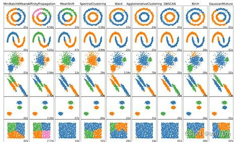
1. Introduction to Common Clustering Algorithms

Clustering is a common unsupervised learning method, which can divide a data set into different classes or clusters according to some specific standards and characteristics, and the data difference in the same class or cluster is as small as possible. Data that are not in the same class or cluster are as diverse as possible.

a. Clustering
The biggest feature of clustering is that the number of clustered clusters is known. It specifies the cluster center point in advance, and through repeated iterations, it finally achieves that the data points in the cluster are close enough and the data between the clusters is close enough. Point to a target far enough away. Common division clusters are: k-means, k-means++, bi-kmeans, etc.

b. Hierarchical clustering
Hierarchical clustering is a clustering analysis method, which gradually merges the objects in the data set into different hierarchical structures according to the similarity. In hierarchical clustering, each data point is initially treated as a single cluster, and then they are merged into larger clusters until all data points are assigned to a single cluster.
There are two different methods of hierarchical clustering: Agglomerative and Divisive. In agglomerative clustering, each data point is initially treated as a separate cluster, and then the clusters are merged by computing the similarity between them. Eventually a large cluster is formed. In divisive clustering, all data points are treated as one large cluster, and then the clusters are split by computing the dissimilarity between them, eventually forming a set of small clusters

c. Density clustering
Density clustering is a clustering method based on the density between data points, whose goal is to group data points with high density and separate them from other data points in low density areas . In density clustering, the density of data points is determined by counting the number of neighbors around each data point. Points with a sufficiently high density are considered "core points", while those without enough neighbors around them are considered "noise points". Density clustering forms clusters by finding core points and their neighbors. The number and shape of clusters are controlled based on threshold settings for density and distance. Density clustering is a non-parametric clustering method that can cluster data without prior determination of the number of clusters, and is suitable for data sets with complex structures and noises. The common density clustering algorithm has DBSCAN algorithm

2. Mathematical principles of two kinds of clustering

1. K-MEANS clustering

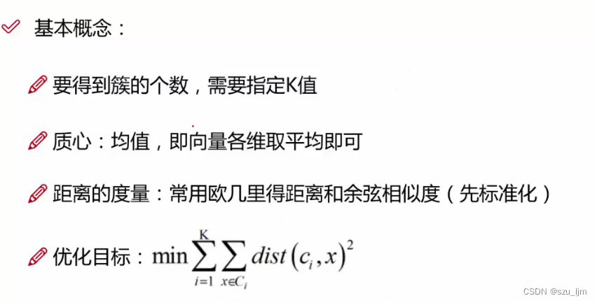
a. Classification of sample points

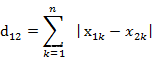
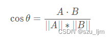
Suppose we have a lot of sample point data in hand, but we don't know their labels. First of all, we need to determine the number of clusters kk after clustering$k$ , and then randomly generate kkon the plane of the same dimension$k$ centroids, or we can also specify an initial vector of centroids. Then we need to measure the distance from each sample point to different centroids, use this distance to measure which centroid is more similar to the sample point, and classify the point into the cluster closest to him. Common distance measurement methods are :

Euclidean distance

Manhattan distance

cosine similarity(Think of a sample data as a vector)

b. Centroid update iteration

When all data sample points are clustered into different clusters, the centroid needs to be updated once, and the mean value of all sample point vectors in the cluster is calculated in different dimensions. The mean value of each dimension is the updated centroid vector ci $c_i$, of which $i$ is the$i$ clusters,$n$ represents the different dimensions of the vector

$$\overrightarrow{c_i}=(\frac{{\sum }_{j=1}^{m_i}{x}_{ij}^1}{m_i}，\frac{{\sum }_{j=1}^{m_i}{x}_{ij}^2}{m_i}，\frac{{\sum }_{j=1}^{m_i}{x}_{ij}^3}{m_i}，\cdots ，\frac{{\sum }_{j=1}^{m_i}{x}_{ij}^n}{m_i})，i=1，2，3，\cdots ,k$$

After the centroid is updated, continue to iterate these two steps, first classify the sample points again, then update the centroid, and finally iterate until the loss function value basically stabilizes and then stop. This is the mathematical principle of K-MEANS clustering implementation.

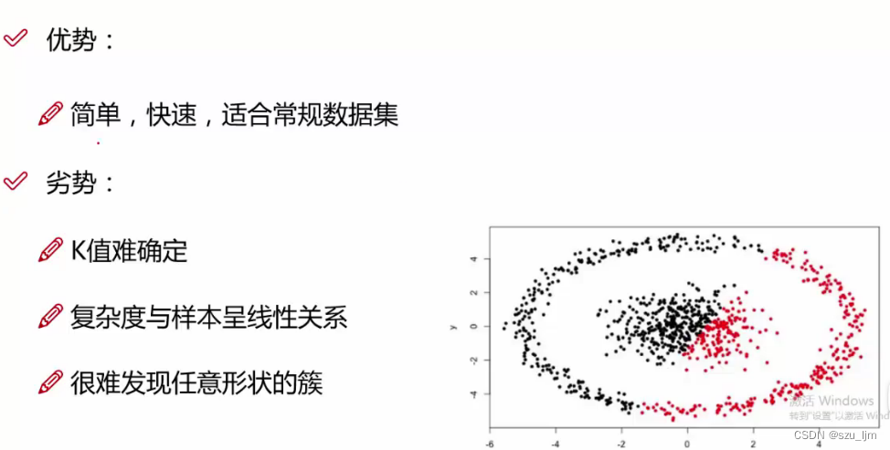
The advantage of K-MEANS clustering algorithm is that it is fast and simple to implement, and it is more suitable for conventional basic data sets. However, once the distribution of data sets is more complicated, the effect of K-MEANS clustering is far inferior to that of DBSCAN clustering. Moreover, the result of K-MEANS clustering has a great correlation with the selection of the initial K value and the selection of the initial centroid position, and the effect of poor selection is not satisfactory.

2. DBSCAN clustering

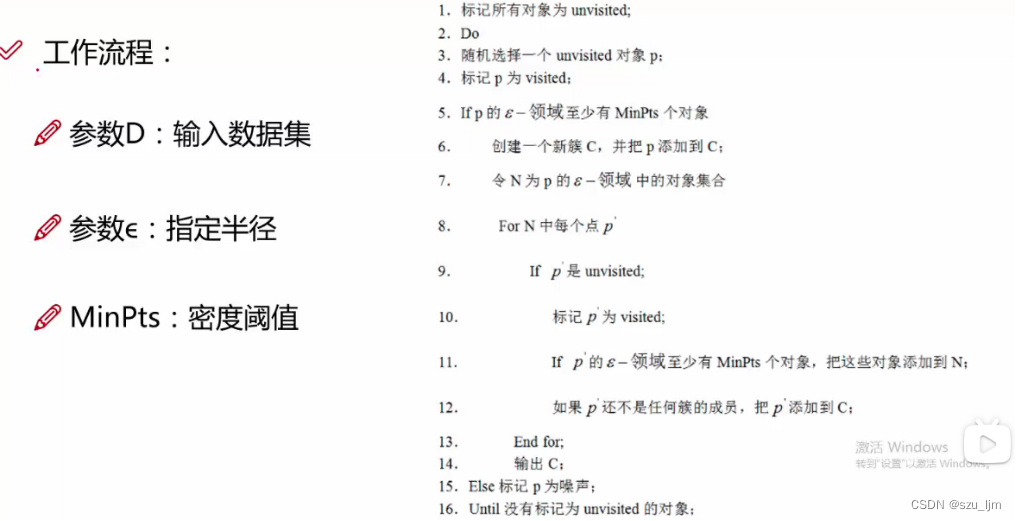
DBSCAN clustering is clustering based on density accessibility, mathematically if a point $p$ at point$qrr$ _$In\; the\; neighborhood\; of\; r$ , that is, the components of the vectors formed by the two points in each dimension are less than or equal to$r$ , this is the direct density reachable

Suppose we have$For\; m$ sample points, first randomly select a sample point as a starting point of a cluster, and then use a given threshold$r$ and feature dimension$n$ scans, including the sample points that enter the scanning range, the scanned sample points will be used as the new starting point for the next scan, and so on, until the number of sample points in the cluster no longer increases, and then proceed to the next cluster clustering of

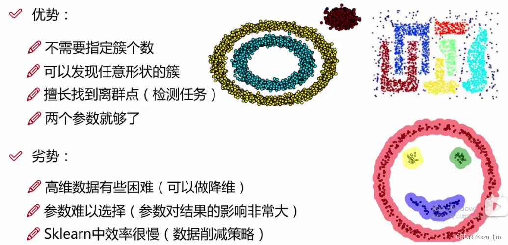
Compared with K-MEANS clustering, DBSCAN clustering has many advantages. For example, it can handle data sets with complex distribution, and is good at finding outliers and noise points. Because there is no need to specify the number of clusters, the effect of DBSCAN clustering will only be Affected by the cluster radius. However, if the clustering radius is not selected properly, it will also affect the results of DBSCAN clustering. It is best to experiment several times and draw the loss function under different radii to obtain the optimal solution.

3. Two Evaluation Metrics

The inertia index can be used to measure the clustering effect of the K-MEANS algorithm, which represents the sum of the distances from each sample point to the centroid of its cluster. According to the definition of inertia, the smaller the inertia, the better, but in fact we can find that when the number of clusters increases, the value of inertia will naturally become smaller and smaller. Even in extreme cases, when the number of clusters is equal to the number of samples, each sample is a cluster, then inertia is 0. Therefore, although inertia is a good measurement standard, it is difficult to define the optimal clustering effect. After all, it is difficult for us to specifically measure the clustering effect without supervision.

$$s(i)=\frac{b(i)-a(i)}{\max ((a(i),b(i)))}$$

Silhouette coefficient $s\left(i\right)$ is an index used to evaluate the clustering effect. It can be understood as an index describing the sharpness of the outline of each category after clustering. It contains two factors - cohesion and separation. Cohesion can be understood as reflecting the closeness of a sample point to elements within the class, and separation can be understood as reflecting the closeness of a sample point to elements outside the class. where$a\left(i\right)$ represents sample$The\; average\; distance\; from\; i$ to other samples of the same cluster, where$b\left(i\right)$ represents sample$The\; average\; distance\; of\; i$ to other samples from another cluster.This $The\; closer\; s\left(i\right)$ is to 1, the higher the density of the cluster where the sample is located, the better the clustering effect; whens ( i ) s(i)The closer$s$$($$i$$)$ is to 0, it means that the sample is at the edge of the cluster; when s ( i ) s(i)The closer s$($$i$$)$$is\; to\; -1,\; the\; lower\; the\; density\; of\; the\; cluster\; where\; the\; sample\; is\; located,\; the\; poorer\; the\; clustering\; effect,\; and\; it\; is\; very\; likely\; that\; the\; sample\; point\; is\; clustered\; wrongly$

---

3. Python implements clustering algorithm

1. K-MEANS clustering and evaluation

To implement K-MEANS clustering in Python, first import several commonly used libraries and generate several block data groups. You can specify the center of the block, the amount of data, the degree of dispersion of distribution and the number of blocks by yourself, and then define the centroid drawing function and data sample points Draw the function, then define the decision boundary drawing function, including drawing the chessboard, classification boundary and centroid drawing function calls, then instantiate K-MEANS and train the model, instantiate the number of clusters to be formulated, centroid initialization status and iteration The number of times, and finally we import the silhouette coefficient as an indicator to measure the clustering effect of K-MEANS in a given number of different clusters

import numpy as np
import matplotlib.pyplot as plt
from sklearn.datasets import make_blobs
from sklearn.cluster import KMeans
from sklearn.metrics import silhouette_score

k = 5
kmeans_per_k = []

blob_centers = np.array([[0.3, 1.1], [-0.2, -0.4], [0.6, -1.8], [1.3, 0.2], [-1.0, 0.8]])
blob_std = np.array([0.32, 0.25, 0.18, 0.12, 0.12])
x, y = make_blobs(n_samples=3000, centers=blob_centers, cluster_std=blob_std, random_state=6)

def plot_clusters(x, y=None):
    plt.plot(x[:, 0], x[:, 1], 'k.', markersize=2)
    plt.xlabel("x_1", fontsize=12)
    plt.xlabel("x_2", fontsize=12)



def plot_centroids(centroids, circle_color='w', cross_color='w'):
    plt.scatter(centroids[:, 0], centroids[:, 1], marker='o', s=10, linewidths=6, color=circle_color, zorder=10, alpha=0.8)
    plt.scatter(centroids[:, 0], centroids[:, 1], marker='x', s=18, linewidths=20, color=cross_color, zorder=10, alpha=1)


def plot_decision_boundaries(clusterer, X, resolution=2000, show_centroids=True):
    mins = X.min(axis=0) - 0.1
    maxs = X.max(axis=0) + 0.1
    xx, yy = np.meshgrid(np.linspace(mins[0], maxs[0], resolution), np.linspace(mins[1], maxs[1], resolution))
    Z = clusterer.predict(np.c_[xx.ravel(), yy.ravel()])
    Z = Z.reshape(xx.shape)
    plt.contourf(Z, extent=(mins[0], maxs[0], mins[1], maxs[1]), camp="Pastel2")
    plt.contour(Z, extent=(mins[0], maxs[0], mins[1], maxs[1]), linewidths=1, color='k')
    plot_clusters(X)
    if show_centroids:
        plot_centroids(clusterer.cluster_centers_)


kmeans = KMeans(n_clusters=k, init='random', n_init=5, random_state=2000)


kmeans_per_k = [KMeans(n_clusters=i).fit(x) for i in range(2, 8)]
y_pred = kmeans.fit(x)
silhouette_score(x, kmeans.labels_)
silhouette_scores = [silhouette_score(x, model.labels_) for model in kmeans_per_k[1:]]


plt.figure(figsize=(12, 8))
plt.subplot(121)
plot_decision_boundaries(kmeans, x)
plt.subplot(122)
plt.plot(range(2, 7), silhouette_scores, 'go--')
plt.show()

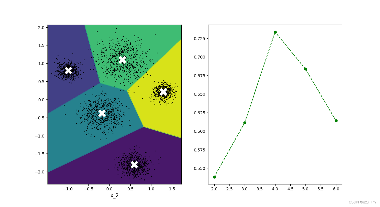
From the line chart of the silhouette coefficient, it can be seen that the optimal number of clusters is around 4, but the number of data blocks we artificially set is 5, so the silhouette coefficient can only be used as a reference index to help you estimate the optimal K value

2. K-MEANS clustering versus DBSCAN clustering

The implementation of DBSCAN clustering in Python is similar to K-MEANS clustering. Here we compare a more complex data set similar to the moon. DBSCAN clustering drawing needs to draw the distribution of sample points, noise points and cluster scanning boundaries. When instantiating, it needs Pass in the cluster radius and the minimum number of sample points for the cluster, and perform model training after instantiation

import numpy as np
import matplotlib.pyplot as plt
from sklearn.datasets import make_moons
from sklearn.cluster import KMeans
from sklearn.cluster import DBSCAN

k = 2


blob_centers = np.array([[0.3, 1.1], [-0.2, -0.4], [0.6, -1.8], [1.3, 0.2], [-1.0, 0.8]])
blob_std = np.array([0.32, 0.25, 0.18, 0.12, 0.12])
x, y = make_moons(n_samples=3000, noise=0.1, random_state=56)

def plot_clusters(x, y=None):
    plt.plot(x[:, 0], x[:, 1], 'b.', markersize=2)
    plt.xlabel("x_1", fontsize=12)
    plt.ylabel("x_2", fontsize=12)



def plot_centroids(centroids, circle_color='w', cross_color='w'):
    plt.scatter(centroids[:, 0], centroids[:, 1], marker='o', s=10, linewidths=6, color=circle_color, zorder=10, alpha=0.8)
    plt.scatter(centroids[:, 0], centroids[:, 1], marker='x', s=18, linewidths=20, color=cross_color, zorder=10, alpha=1)


def plot_decision_boundaries(clusterer, X, resolution=2000, show_centroids=True):
    mins = X.min(axis=0) - 0.1
    maxs = X.max(axis=0) + 0.1
    xx, yy = np.meshgrid(np.linspace(mins[0], maxs[0], resolution), np.linspace(mins[1], maxs[1], resolution))
    Z = clusterer.predict(np.c_[xx.ravel(), yy.ravel()])
    Z = Z.reshape(xx.shape)
    plt.contourf(Z, extent=(mins[0], maxs[0], mins[1], maxs[1]), camp="Pastel2")
    plt.contour(Z, extent=(mins[0], maxs[0], mins[1], maxs[1]), linewidths=1, color='k')
    plot_clusters(X)
    plt.title("K-MEANS")
    if show_centroids:
        plot_centroids(clusterer.cluster_centers_)


def plot_dbscan(dbscan, X, size):
    core_mask = np.zeros_like(dbscan.labels_, dtype=bool)
    core_mask[dbscan.core_sample_indices_] = True
    anomalies_mask = dbscan.labels_ == -1
    non_core_mask = ~(core_mask | anomalies_mask)

    cores = dbscan.components_
    anomalies = X[anomalies_mask]
    non_cores = X[non_core_mask]

    plt.scatter(cores[:, 0], cores[:, 1], c=dbscan.labels_[core_mask], marker='o', s=size, cmap="Paired")
    plt.scatter(cores[:, 0], cores[:, 1], c=dbscan.labels_[core_mask], marker='*', s=15)
    plt.scatter(anomalies[:, 0], anomalies[:, 1], c='r', marker='x', s=100)
    plt.scatter(non_cores[:, 0], non_cores[:, 1], c=dbscan.labels_[non_core_mask], marker='.')
    plt.xlabel("x_1", fontsize=12)
    plt.ylabel("x_2", fontsize=12)
    plt.title("DBSCAN")






kmeans = KMeans(n_clusters=k, init='random', n_init=5, random_state=2000)
dbscans = DBSCAN(eps=0.1, min_samples=10)


y_kmeans_pred = kmeans.fit(x)
y_dbscan_pred = dbscans.fit(x)



plt.figure(figsize=(12, 8))
plt.subplot(121)
plot_decision_boundaries(kmeans, x)
plt.subplot(122)
plot_dbscan(dbscans, x, size=200)
plt.show()

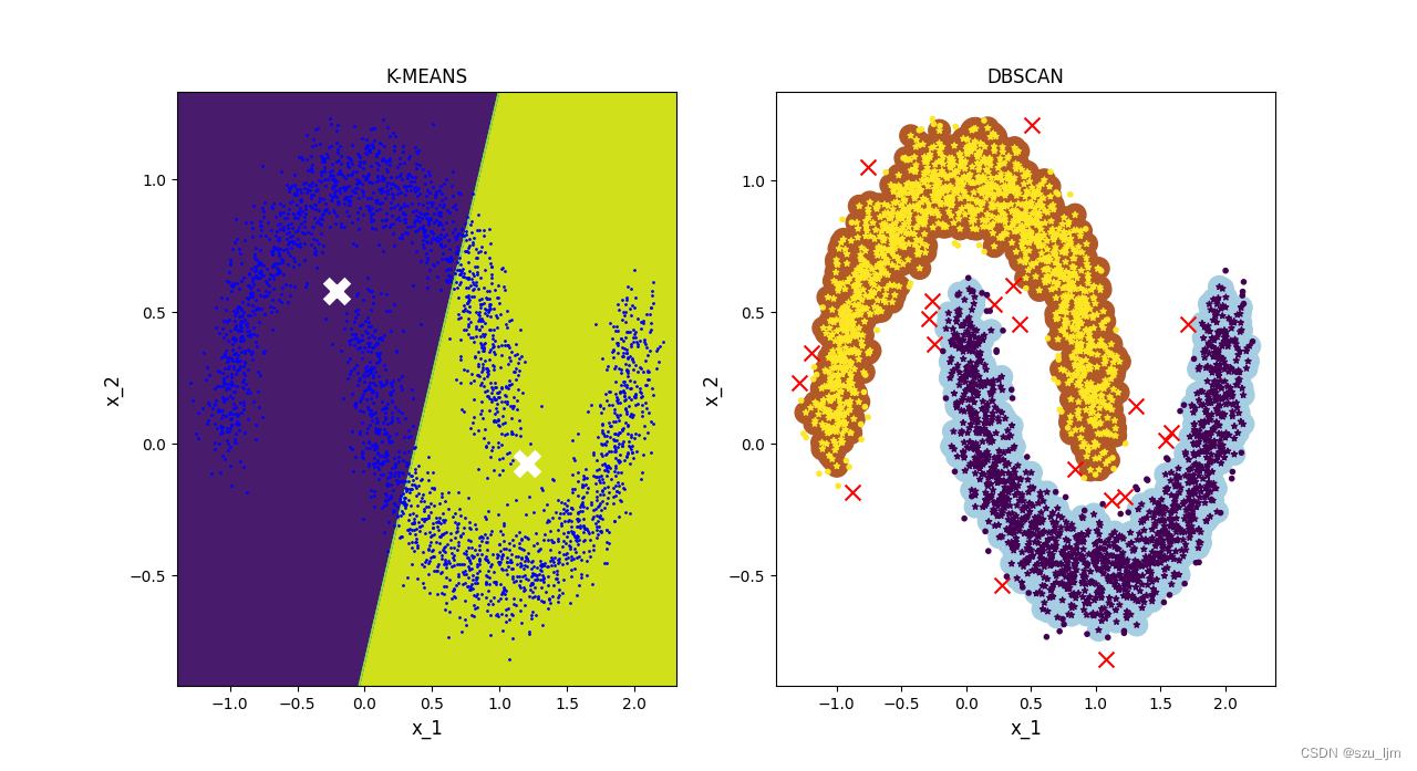
From the above two figures, it can be clearly seen that the effect of DBSCAN clustering is much better than that of K-MEANS clustering when dealing with complex distribution data sets, and DBSCAN clustering is good at finding outliers, and is doing detection tasks. more useful when

3. K-MEANS image segmentation

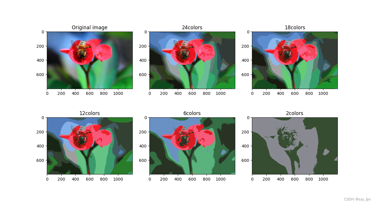
The core principle of K-MEANS image segmentation is clustering based on distance. An image data is composed of length, width and color channel number. Each corresponding pixel will store three components of RGB, and each element of the RGB matrix is ​​taken as Value range is $[0,255]$ , different RGB permutations and combinations can form$2^{24}$ colors, which restore the colors our human eyes see in real life. K-MEANS image segmentation is to cluster the number of color channels of each pixel according to the number of given clusters, and fill the pixels of the same cluster as the RGB three component values ​​of the centroid of the cluster

import matplotlib.pyplot as plt
from matplotlib.image import imread
from sklearn.cluster import KMeans

image = imread("flower.jpg")
image = image / 255
division_images = []

x = image.reshape(-1, 3)


n_colors = (24, 18, 12, 6, 2)

for n_cluster in n_colors:
    kmean = KMeans(n_clusters=n_cluster, random_state=42).fit(x)
    division_image = kmean.cluster_centers_[kmean.labels_]
    division_images.append(division_image.reshape(image.shape))


plt.figure(figsize=(12, 8))
plt.subplot(231)
plt.imshow(image)
plt.title('Original image')
for index, n_clusters in enumerate(n_colors):
    plt.subplot(232+index)
    plt.imshow(division_images[index])
    plt.title('{}colors'.format(n_clusters))

plt.show()

Summarize

The above are the study notes of the machine learning clustering algorithm. This note simply records the mathematical principle of the clustering algorithm and the idea of ​​​​Python implementation. Although the implementation effect of the clustering algorithm is not as good as that of the classification algorithm in most cases, after all, clustering is Unsupervised learning and classification is supervised learning, but clustering algorithms can still play an advantage in specific application cases, not as good as K-MEANS clustering in image segmentation. In short, we need to master the advantages of different algorithms , Make use of strengths and avoid weaknesses, complement each other!