Getting Started with Python Machine Learning - Decision Tree Algorithm Study Notes

Tip: After the article is written, the table of contents can be automatically generated. How to generate it can refer to the help document on the right

---

foreword

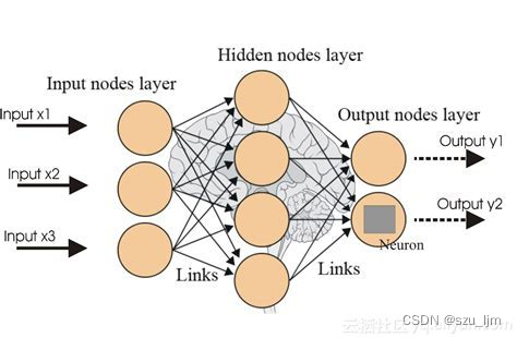
As soon as ChatGPT came out, it brought a huge shock and impact to the whole society. People can't help but marvel at the power of AI now, and we seem to be one step closer to general artificial intelligence. In the vigorous development of the field of artificial intelligence in the past ten years, the algorithms that play a dominant role are basically neural networks and deep learning, and many machine learning algorithms have been eclipsed. Although neural networks and deep learning are powerful, it is difficult for us to explain what is inside this "black box". Just like the human brain, the interaction between neurons is very complex and subtle. Is there a more powerful model in machine learning that can be explained well? Yes, that is the integrated learning algorithm random forest, and each individual classifier of the random forest is our protagonist today - the decision tree.

1. Introduction to Decision Tree Algorithm

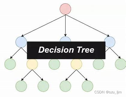
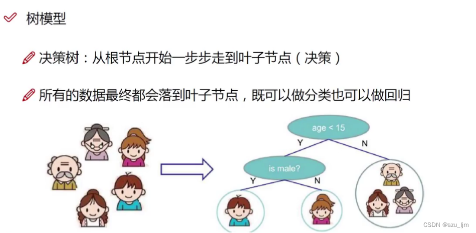
Decision tree algorithm is a commonly used supervised learning machine learning algorithm, and it is a predictive analysis model expressed in the form of tree structure (including binary tree and multi-fork tree).A tree is a special data structure, a directed acyclic graph, that is, a tree has a direction but does not form a closed-loop graph, and its main function is to classify and traverse. The decision tree uses the idea of ​​classification to construct a mathematical model according to the characteristics of the data, so as to achieve the screening of data and complete the goal of decision-making. Each node in the decision tree represents a feature object, and each branch path represents a possible classification method, and each leaf node corresponds to the object represented by the path from the root node to the leaf node. value.

2. Mathematical principle of decision tree

The decision tree algorithm is a model for the purpose of classification. This classification aims to reduce the entropy value of the sample labels in each class, that is, to make the labels of the sample data in this class more consistent. After transformation, we can also apply the decision tree algorithm In solving the problem of regression prediction

1. The measure of entropy

Entropy is a measure of the uncertainty of random variables. The greater the entropy of things, the greater the chaos of things, and the smaller the entropy of things, the smaller the chaos of things. In the physical world, entropy always tends to increase. conduct. In the decision tree, we use entropy to measure the degree of confusion of the sample labels of the leaf nodes after classification. We hope that the lower the entropy value of the branch nodes, the better, so as to
achieve good results in the decision-making of subsequent leaf nodes.

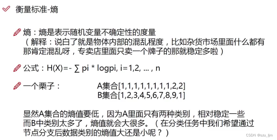
In the branch nodes of the decision tree, we use the proportion of random variables to measure the probability of its occurrence according to the classical concept, and convert the probability value into information entropy, H ( X ) H(X $H\left(X\right)$ means information entropy value
$$H(X)=-\sum _{i=1}^n{p}_{i}log(p_i)$$

In addition to the classic application of information entropy, we sometimes involve the concept of conditional entropy. The relationship between conditional entropy and information entropy is like the relationship between conditional probability and probability. Conditional entropy emphasizes the uncertainty measurement of things under certain conditions, $H(Y|X)$ means conditional entropy
$$H(Y|X)=\sum _{i=1}^n{p}_{i}H(Y|X=x_i)$$
$$H(Y|X=x_i)=\sum _{j=1}^{n}p({and}_j|x=x_i)log(p(y_j|x=x_i))$$

Generally we are calculating $H(Y|X=x_i)$ when we narrow the sample space and use the classical concept to calculate. When the probability in entropy and conditional entropy is obtained by data estimation (especially maximum likelihood estimation), the corresponding entropy and conditional entropy are called empirical entropy and empirical conditional entropy respectively.

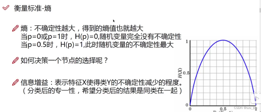
According to the function of entropy $p_{i}log{p}_i$When the probability value of a random variable is close to 1 or 0, that is, the set basically contains this variable or basically does not exist, it means that the uncertainty of the set is very low, and the function value tends to be Near 0, the entropy value approaches 0, and the labels in the set are very orderly; when the probability value of a random variable is distributed between 0 and 1, that is, there is this variable in the set and there are other variables, it means that the set is uncertain At this time, the entropy value is high, and the labels in the collection are disordered

2. Information gain

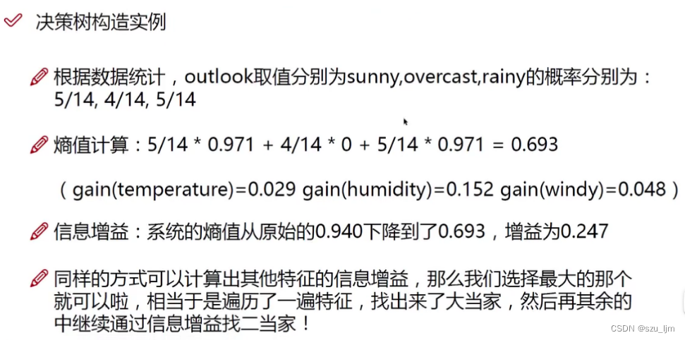
The three common algorithms in the decision tree model are: ID3, C4.5, and CART. The ID3 algorithm uses information gain as the standard to measure which scheme is optimal under different node feature selections, that is, select the node feature with the largest information gain in a circular manner, and then recursively go down to form a decision tree, using the feature $a$ pair sample setDDThe "information gain" obtained by dividing$D$
$$InfoGain(D|a)=H(D)-H(D|a)$$
Then we select the feature node with the largest information gain, and then recursively traverse the next node. To put it simply, we use the information gain method to achieve a more orderly effect of node labels and enhance the certainty of leaf nodes, just like shopping websites classify products, first divide digital area supplies, daily necessities, etc., and then classify them by brand or price sort

The C4.5 algorithm uses the information gain rate as a standard, and considers the influence of its own entropy value more than the ID3 algorithm. If the decision tree has more categories, and each sub-node is assigned, the purity of the sub-nodes will also increase. The more likely it is, because the number is less, it may be the most likely to be in a class, and even a leaf node can have a label value, but this will make the decision tree model overfit, so we reduce the consideration of introducing our own attributes. Fitting risk
$$GainRatio(D|a)=-\frac{InfoGain(D|a}{H(D|a)}$$

The purity of node labels in the CART algorithm can be measured by the Gini value, and the Gini coefficient reflects the probability that two samples are randomly drawn from the data set D, and their category labels are inconsistent. Therefore, the smaller the Gini coefficient, the higher the purity of the node
$$Gini(p)=\sum _{k=1}^n{p}_k(1-p_k)$$

3. Pruning strategy

The pruning strategy aims to reduce the risk of over-fitting of the decision tree and limit the complexity of the decision boundary. To put it bluntly, there are too many branches and leaves in your garden. At this time, you need to prune these branches and leaves to make the tree look more refreshed and energized

The pruning strategy of the decision tree is divided into pre-pruning and post-pruning. Pre-pruning is relatively simple, which is to limit the depth of the tree and the number of leaf nodes before the decision tree is generated, so as to avoid the situation that one leaf node has one label value. , which is equivalent to the tree in your home while you are growing and you are pruning the branches and leaves

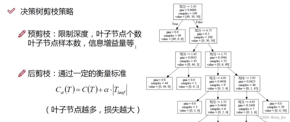
The post-pruning of the decision tree is to prune the tree model after the decision tree is generated. The cost complexity pruning-CCP uses $C\left(T\right)$ is used as a loss function to measure the effect of the decision tree, where$T$ is the number of leaf nodes. This involves an important parameter$\alpha$ ,$\alpha$ is given by itself,$The\; larger\; the\; \alpha$ , the less you want the tree model to overfit,α \alphaThe smaller$the\; \alpha \; ,\; the\; more\; you\; want\; the\; classification\; effect\; of\; the\; decision\; tree\; to\; be\; better,\; that\; is,\; the\; higher\; the\; purity\; of\; the\; leaf\; nodes$

3. Python implements decision tree algorithm

1. CART decision tree

The idea of ​​​​Python to implement the decision tree algorithm is the same as before. First, import the commonly used packages and the iris data set, then select several features and labels of the iris data and instantiate the decision tree, train the decision tree, and then display it with the graphviz tool Decision tree, and use matplotlib to draw the board and decision boundary, and finally show it

import numpy as np
from sklearn.datasets import load_iris
from sklearn.tree import DecisionTreeClassifier
from sklearn.tree import export_graphviz
from IPython.display import Image
from matplotlib.colors import ListedColormap
import matplotlib.pyplot as plt

iris = load_iris()
x = iris.data[:, 2:]
y = iris.target

tree_clf = DecisionTreeClassifier(max_depth=2)
tree_clf.fit(x, y)

def plot_decision_boundary(clf, x, y, axes=[0, 7.5, 0, 3]):
    x1a = np.linspace(axes[0], axes[1], 100)
    x2a = np.linspace(axes[2], axes[3], 100)
    x1, x2 = np.meshgrid(x1a, x2a)
    x_new = np.c_[x1.ravel(), x2.ravel()]
    y_pred = clf.predict(x_new).reshape(x1.shape)
    custom_cmap = ListedColormap(['#fafab0', '#9898ff', '#507d50'])
    plt.contourf(x1, x2, y_pred, alpha=0.3, cmap=custom_cmap)
    plt.plot(x[:, 0][y == 0], x[:, 1][y == 0], "yo", label="Iris-Setosa")
    plt.plot(x[:, 0][y == 1], x[:, 1][y == 1], "bs", label="Iris-Versicolor")
    plt.plot(x[:, 0][y == 2], x[:, 1][y == 2], "g^", label="Iris-Virginica")
    plt.axis(axes)
    plt.xlabel("Petal length", fontsize=12)
    plt.ylabel("Petal width", fontsize=12)


export_graphviz(tree_clf, out_file="iris_tree.dot", feature_names=iris.feature_names[2:], class_names=iris.target_names, rounded=True, filled=True )
plt.figure(figsize=(12, 8))
plot_decision_boundary(tree_clf, x, y)
plt.plot([2.45, 2.45], [0, 3], "k-", linewidth=2)
plt.plot([2.45, 7.5], [1.75, 1.75], "k--", linewidth=2)
plt.plot([4.95, 4.95], [0, 1.75], "k:", linewidth=2)
plt.plot([4.85, 4.85], [1.75, 3], "k:", linewidth=2)
plt.text(1.4, 1.0, "Depth=0", fontsize=15)
plt.text(3.2, 1.8, "Depth=1", fontsize=13)
plt.text(4.05, 0.5, "Depth=2", fontsize=11)
plt.title('Decision Tree')
plt.show()

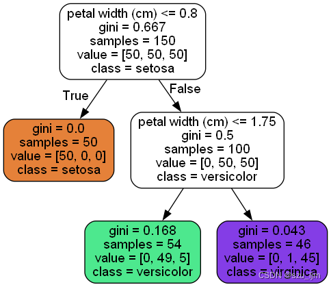
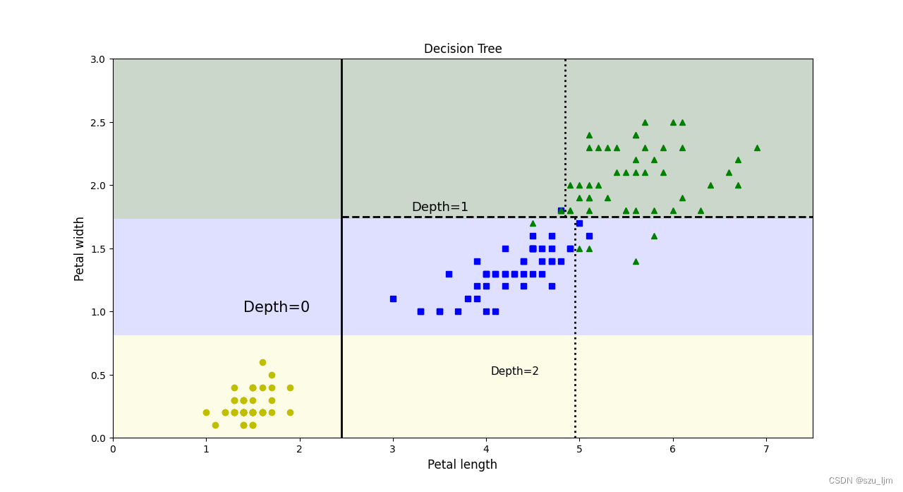
Decision trees can be seen via $The$$Gini$ coefficient is used as the criterion for judging the effect of node classification. First, the first type of flowers is completely separated with the petal width of 0.8 as the boundary, and then the remaining two kinds of flowers are basically separated with the petal width of 1.75 as the petal width.

2. Decision tree pruning comparison

The idea of ​​implementing decision tree pruning comparison in Python is the same as before. First import commonly used packages and moon data sets, specify the number of samples and noise rate of the moon data set, then instantiate and train the decision tree, and then use matplotlib Draw the chessboard and decision boundary, and finally use two subgraphs to show two different effects

import numpy as np
import matplotlib.pyplot as plt
from sklearn.datasets import make_moons
from sklearn.tree import DecisionTreeClassifier
from matplotlib.colors import ListedColormap

x, y = make_moons(n_samples=200, noise=0.3, random_state=50)
tree_clf1 = DecisionTreeClassifier(random_state=50)
tree_clf2 = DecisionTreeClassifier(min_samples_leaf=9, random_state=50)
tree_clf1.fit(x, y)
tree_clf2.fit(x, y)

def plot_decision_boundary(clf, x, y, axes=[0, 7.5, 0, 3]):
    x1a = np.linspace(axes[0], axes[1], 100)
    x2a = np.linspace(axes[2], axes[3], 100)
    x1, x2 = np.meshgrid(x1a, x2a)
    x_new = np.c_[x1.ravel(), x2.ravel()]
    y_pred = clf.predict(x_new).reshape(x1.shape)
    custom_cmap = ListedColormap(['#fafab0', '#9898ff', '#507d50'])
    plt.contourf(x1, x2, y_pred, alpha=0.3, cmap=custom_cmap)
    plt.plot(x[:, 0][y == 0], x[:, 1][y == 0], "yo", label="Iris-Setosa")
    plt.plot(x[:, 0][y == 1], x[:, 1][y == 1], "bs", label="Iris-Versicolor")
    plt.plot(x[:, 0][y == 2], x[:, 1][y == 2], "g^", label="Iris-Virginica")
    plt.axis(axes)
    plt.xlabel("Petal length", fontsize=12)
    plt.ylabel("Petal width", fontsize=12)


plt.figure(figsize=(12, 8))
plt.subplot(121)
plot_decision_boundary(tree_clf1, x, y, axes=[-1.5, 2.5, -1, 1.5])
plt.title("No restrction")
plt.subplot(122)
plot_decision_boundary(tree_clf2, x, y, axes=[-1.5, 2.5, -1, 1.5])
plt.title("min_slamples=9")
plt.show()

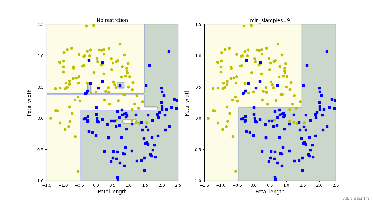
We can see that the decision boundary without pruning is very complex, and the risk of over-fitting is extremely high; while the decision boundary after pruning and the minimum number of leaf node samples is relatively simple, the risk of over-fitting is low, and when dealing with noise Doing well on this

Summarize

The above are the study notes of the decision tree algorithm in machine learning. This note briefly introduces the mathematical principles and program ideas of the decision tree. Decision tree can be regarded as a model that is very easy to explain in machine learning. The machine learning integration algorithm random forest in the next note is also an extension and extension of decision tree. Integration algorithm still has a place today when deep learning is widely touted. It is inseparable from the powerful interpretability and generalization capabilities of decision trees.