In this project, we will learn how to use a Convolutional Variational Autoencoder (CVAE) to process and reconstruct 3D turbulence data.
We use computational fluid dynamics (CFD) methods to generate 3D turbulent cubes, each of which carries physical information along three velocity components (similar to image data, treated as separate channels).

Recommendation: Use NSDT Designer to quickly build programmable 3D scenes.
As part of 3D CFD data preprocessing, we wrote a custom pytorch data loader to perform normalization and batch operations on the dataset.
CVAE implements 3D convolutions (3DConvs) on preprocessed data to perform reconstruction.
By fine-tuning hyperparameters and manipulating our model architecture, we achieve significant improvements in 3D reconstruction.
The project code can be found in this Github repository .
1. Data description
Our dataset was generated using CFD simulations and consists of cubes extracted from heating ventilation and air conditioning (HVAC) ducts.
Each cube represents a three-dimensional temporal snapshot of the turbulent flow carrying physical information at a specific time. The information extracted from the simulation is based on two flow components: the velocity field U and the static pressure p. The U field (x, y, z) and the scalar p are based on the direction of the flow (the normal direction of the cube).
We represent a 3D cube using voxels as an array of size 21 × 21 × 21 x 100 (x_coord, y_coord, z_coord, timestep). The figure below shows a cube data sample where we visualize each velocity component using a heatmap.
In total, the dataset consists of 96 simulations with 100 time steps each, for a total of 9600 cubes (for each velocity component).

NOTE: Due to confidentiality restrictions we do not make our data public, you can use the script and adapt it to your own 3D data.
2. Data preprocessing
The script below shows a custom pytorch data loader written for preprocessing 3D data. Here are some highlights:
- Loading and concatenation of cube velocity channels
- data standardization
- data scaling
See the dataloader.py script in the repository for a complete implementation.
3. Model Architecture
The figure below shows the implemented CVAE architecture. In this example, 2DConv is shown for clarity, but the implemented architecture uses 3DConv.
The CVAE consists of an encoder network (top), variational layers (mu and sigma) (middle right), and a decoder network (bottom).
The encoder performs downsampling operations on the input cubes, and the decoder upsamples them to restore the original shape. The variation layer tries to learn the distribution of the dataset, which layer can be used for generation later.
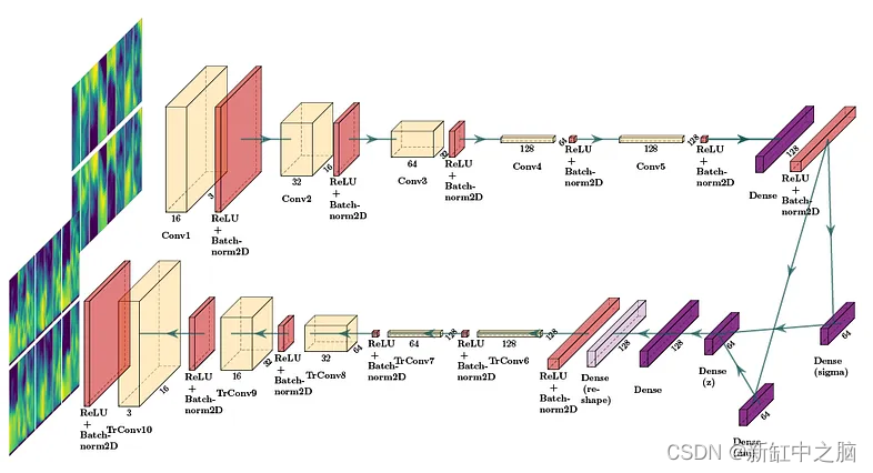
The encoder network consists of four 3D convolutional layers, each with twice the number of convolutional filters than the previous layer (32, 64, 128, and 256, respectively), which enables the model to learn more complex flow features.
A dense layer is used to combine all feature maps obtained from the last encoder layer, which is connected to a variational layer that computes the parameters (mu and sigma) of the distribution of the posterior streaming data using a redefined probability distribution. - The parameterization trick described in [1]. This probability distribution allows us to sample from it to generate a synthetic 3D cube of size 8 x 8 x 8.
The decoder network takes the latent vector and applies four 3D transposed convolutional layers to recover (reconstruct) the original data dimensionality, each layer has half the number of convolutional filters of the previous layer (256, 128, 64 and 32 ).
CVAE is trained using two loss functions: mean squared error (MSE) for reconstruction and Kullback-Leibler divergence (KLB) for latent space regularization.
We use the architecture proposed in [2] and the hyperparameters in [3] as the baseline architecture.
The script below shows an example in pytorch where both the encoder and decoder are defined using 3D convolutional layers (Conv3d):
self.encoder = nn.Sequential(
            nn.Conv3d(in_channels=image_channels, out_channels=16, kernel_size=4, stride=1, padding=0),
            nn.BatchNorm3d(num_features=16),
            nn.ReLU(),
            nn.Conv3d(in_channels=16, out_channels=32, kernel_size=4, stride=1, padding=0),
            nn.BatchNorm3d(num_features=32),
            nn.ReLU(),
            nn.Conv3d(in_channels=32, out_channels=64, kernel_size=4, stride=1, padding=0),
            nn.BatchNorm3d(num_features=64),
            nn.ReLU(),
            nn.Conv3d(in_channels=64, out_channels=128, kernel_size=4, stride=1, padding=0),
            nn.BatchNorm3d(num_features=128),
            nn.ReLU(),
            nn.Conv3d(in_channels=128, out_channels=128, kernel_size=4, stride=1, padding=0),
            nn.BatchNorm3d(num_features=128),
            nn.ReLU(),
            Flatten()
        )

self.decoder = nn.Sequential(
            UnFlatten(),
            nn.BatchNorm3d(num_features=128),
            nn.ReLU(),
            nn.ConvTranspose3d(in_channels=128, out_channels=128, kernel_size=4, stride=1, padding=0),
            nn.BatchNorm3d(num_features=128),
            nn.ReLU(),
            nn.ConvTranspose3d(in_channels=128, out_channels=64, kernel_size=4, stride=1, padding=0),
            nn.BatchNorm3d(num_features=64),
            nn.ReLU(),
            nn.ConvTranspose3d(in_channels=64, out_channels=32, kernel_size=4, stride=1, padding=0),
            nn.BatchNorm3d(num_features=32),
            nn.ReLU(),
            nn.ConvTranspose3d(in_channels=32, out_channels=16, kernel_size=4, stride=1, padding=0),
            nn.BatchNorm3d(num_features=16),
            nn.ReLU(),
            nn.ConvTranspose3d(in_channels=16, out_channels=image_channels, kernel_size=4, stride=1, padding=0), # dimensions should be as original
            nn.BatchNorm3d(num_features=3))
4. Set up the environment
Clone this repository:
git clone [email protected]:agrija9/Convolutional-VAE-for-3D-Turbulence-Data
It is recommended to use a virtual environment to run this project:
- Anaconda can be installed and an environment created in the system
- The environment can be created using pip venv
Install the following dependencies in the pip/conda environment:
- NumPy (>= 1.19.2)
- Matplotlib (>= 3.3.2)
- PyTorch (>= 1.7.0)
- Torchvision (>= 0.8.1)
- scikit-learn (>= 0.23.2)
- tqdm
- tensorboardX
- torchsummary
- PIL
- collections
5. Model training
To train the model, open a terminal, activate the pip/conda environment and type:
cd /path-to-repo/Convolutional-VAE-for-3D-Turbulence-Data
python main.py --test_every_epochs 3 --batch_size 32 --epochs 40 --h_dim 128 --z_dim 64
Following are some hyperparameters that can be modified to train the model
- –batch_size number of cubes to process per patch
- –epochs number of training epochs
- –h_dim hidden dimensions of dense layers (connected to variational layers)
- –z_dim latent space dimension
The main.py script calls the model and trains it on the 3D CFD data. It takes about 2 hours to train for 100 epochs using an NVIDIA Tesla V100 GPU. In this example, the model was trained for 170 epochs.
Note that when training a 3DConvs model, the number of learned parameters increases exponentially compared to a 2DConvs model, and thus, the training time on 3D data is much longer.
6. Model output
After training the pytorch model, a file checkpoint.pkl containing the trained weights will be generated.
During training, every n epochs the model is evaluated against the test data, the script compares the reconstructed cube with the original cube and saves them as images. Additionally, the loss values are recorded and placed in the run folder, and the loss curve can be visualized using tensorboard by typing:
cd /path-to-repo/Convolutional-VAE-for-3D-Turbulence-Data
tensorboard --logdir=runs/
If not created, the folder runs/ will be automatically generated.
7. 3D reconstruction results
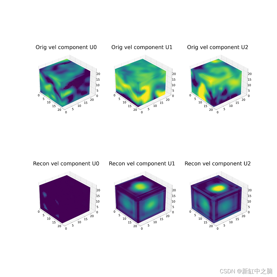
In the figure below, we show the reconstruction results of the same cube sample every n epochs.
The top row contains raw cube samples (for each velocity channel). The bottom row contains the reconstruction output for every n epochs.
For this example, we show reconstructions from 0 to 355 epochs, with intervals of 15 epochs. Note the improvement in reconstruction as a function of epochs.
Original Link: 3D VAE Neural Network Combat—BimAnt