This series can help you improve your skills in using Excel.
Many people think that formulas in Excel are used to produce a single result for a specific cell.
In fact, the dynamic array function of "Excel" can apply the same formula to multiple cells, and perform independent calculations in each cell, thereby completing a large amount of work in a short time, while reducing the possibility of errors lowest. You can use these magic formulas anywhere you need to repeatedly calculate an array of data.
Here are two examples to see how to use the dynamic array function to save time and effort.
Foundation Skills: Creating Addition Tables
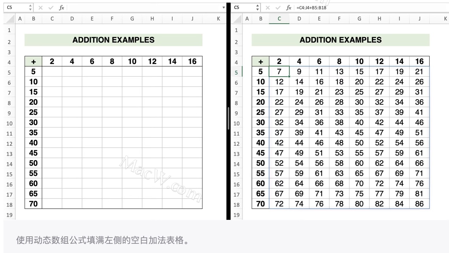
Your goal : Create an addition table similar to the one below to help children learn math and check the results of their operations.
Traditional way: After entering the values to be added in the first row and column, create a formula like =C4+B5 in the first cell, then copy and paste this cell in the entire row, and then copy the entire row Copy it and paste it to other rows of the table. It can be said to be quite troublesome!
"Dynamic" method: create a single formula that references all cells, and calculate the value of each cell at once. Operation method: take the following table as an example, enter =C4:J4+B5:B18 in the first answer cell (C4:J4 represents the range of the first row, B5:B18 represents the range of the first column). Press the Return key and the values will automatically fill the entire table!
Advanced Skill: Summarize Data by Person or by Category
Your goal: In a sales contest, enter data from weekly sales champions, calculate each person's total sales, and update those numbers over time as new champions emerge.
The traditional way: You can use the =SUMIFO function to summarize sales by person, but since new sales champions are determined every week, the range of the table will continue to expand, which means you need to manually adjust the formula every week.
"Dynamic" approach: Use a dynamic array to automatically update the table range when a weekly sales champion joins.
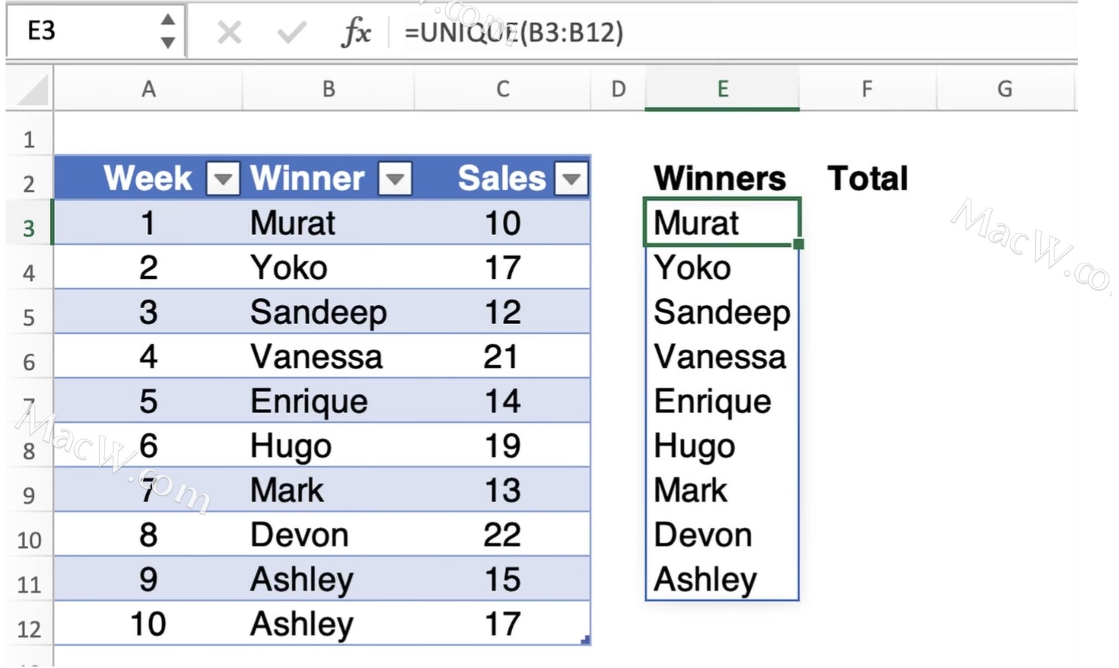
How it works: The table below shows the weekly champion stats so far. Using a new UNIQUE( function, you can easily list the list of salespeople without repeated entry. In a blank area of the workbook, enter the formula =UNIQUE(B3:B12), where B3:B12 is the current list of champions:
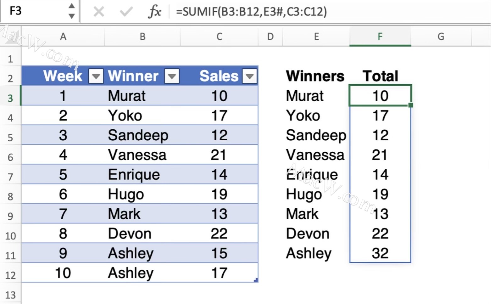
To get the total sales for each person, you need to use a special =SUMIFO function: In the column next to Murat's name, enter the formula
=SUMIF(B3:B12,E3#C3:C12), where B3:B12 is the current list of champions, and c3:C12 is the current list of weekly sales.
The number sign (#) is the key, it allows Excel to refer to the entire range of the dynamic array, ie count any newly added rows. Hit the Return key, and Excel sums up everyone's sales:
Now, assuming Alyssa becomes the top seller for week 11, the relevant data is automatically added to the summary list:

"Excel" provides a variety of ways to use dynamic arrays, including functions such as FILTERO, SORTO, SORTBYO, SEQUENCE() and RANDARRAYO. You only need to use the above function once, and you can fill endless cells, saving precious time.