
本文约4400字,建议阅读9分钟
本文从三个角度与你分享基于反事实因果推断的度小满额度模型。
1. The research paradigm of causal inference
(1) Correlation and causation
(2) Three basic assumptions
2. Framework evolution of causal inference
(1) From random data to observed data
(2) Counterfactual Representation Learning
3. Counterfactual Quota Model Mono-CFR
(1) The counterfactual estimation problem of continuous Treatment
Sharing guests|Wan Shi Xiang Du Xiaoman Expert Algorithm Engineer
Editing|Xu Yiyi Bytedance
Production Community|DataFun
01 Research paradigm of causal inference
There are currently two main research directions in the research paradigm:
Judea Pearl Structure Model
potential output frame
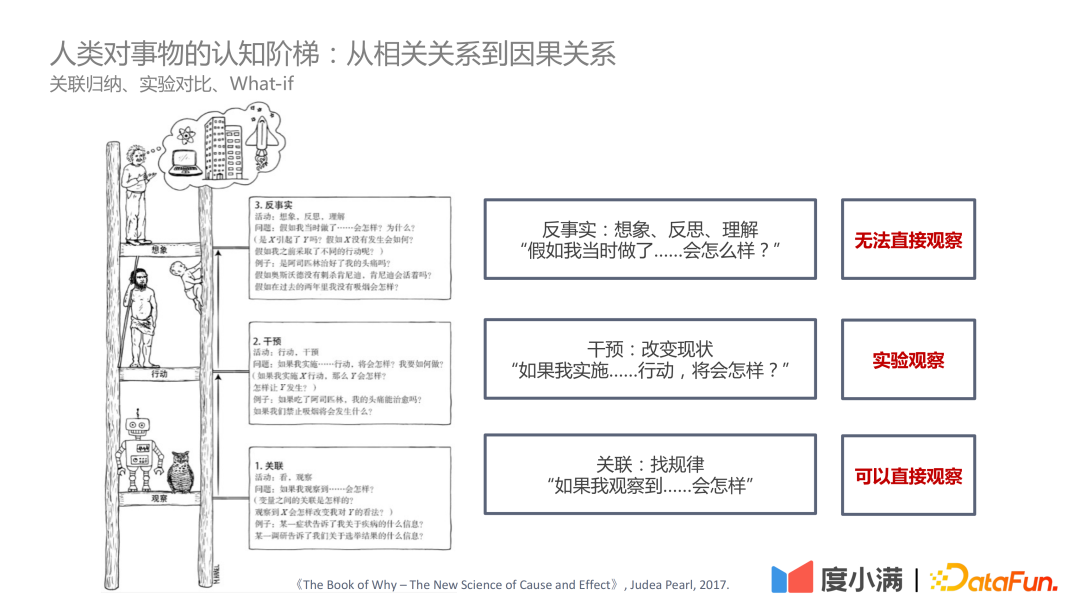
In the book "The Book of Why – The New Science of Cause and Effect" by Judea Pearl, the cognitive ladder is positioned as three levels:
The first layer - correlation: find out the law through the correlation method, which can be directly observed;
The second layer-intervention: if the status quo is changed, what actions should be implemented and what conclusions should be drawn, which can be observed through experiments;
The third layer-counterfactual: Since laws and regulations and other issues cannot be directly observed experimentally, what will happen if an action is implemented through counterfactual assumptions, and how to evaluate ATE and CATE is a relatively difficult problem.
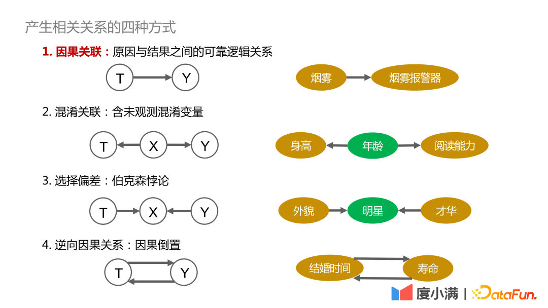
First, the four ways to generate correlations are described below:
1. Causal relationship: There is a reliable, traceable, and positively dependent relationship between the cause and the effect, such as the causal relationship between smoke and smoke alarms;
2. Confused correlation: Confounding variables that cannot be directly observed, such as whether height and reading ability can be related, need to control the variable of age to draw valid conclusions;
3. Selection bias: It is Berkson’s paradox in essence, such as exploring the relationship between appearance and talent. If you only observe in the star group, you may come to the conclusion that you cannot have both appearance and talent. If observed in all human beings, there is no causal relationship between appearance and talent.
4. Reverse causality: the inversion of causality. For example, statistics show that the longer a human is married, the longer his life expectancy. But conversely, we cannot say: if you want to get a longer life span, you have to get married early.
How the confusion factor affects the observation results, here are two cases to illustrate:
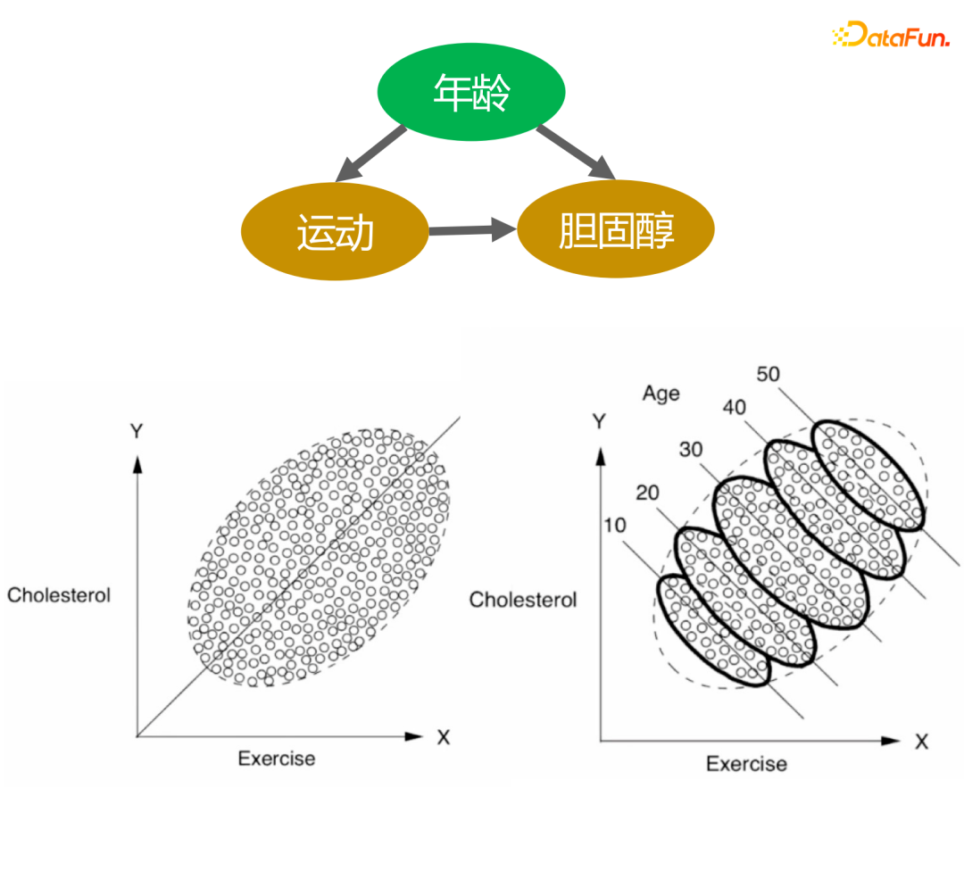
The picture above depicts the relationship between exercise and cholesterol levels. From the graph on the left, it can be concluded that the greater the amount of exercise, the higher the cholesterol level. However, looking at age stratification, under the same age stratification, the greater the amount of exercise, the lower the cholesterol level. In addition, with age, cholesterol levels gradually increase, this conclusion is in line with our cognition.

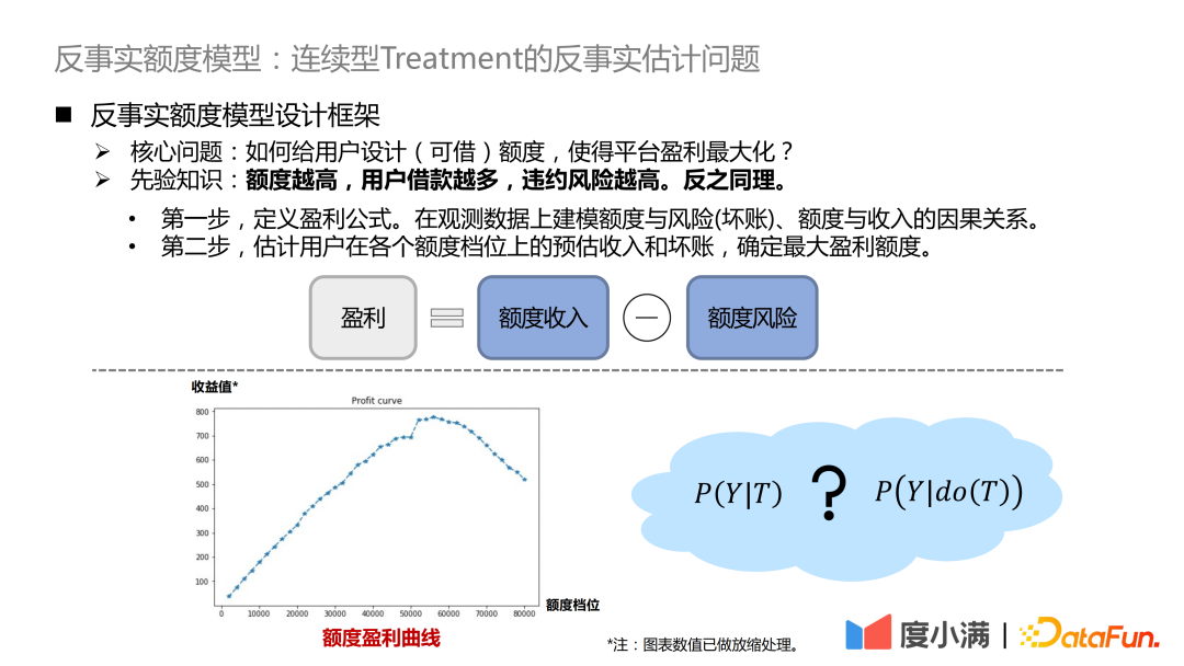
The second example is the credit scenario. It can be seen from historical statistics that the higher the given amount (the amount of money that can be borrowed), the lower the overdue rate. However, in the financial field, the credit qualification of the borrower will be judged first based on the A-card of the borrower. If the credit qualification is better, the amount granted by the platform will be higher, and the overall overdue rate will be low. However, according to local random experiments, among people with the same credit qualifications, some people’s quota risk migration curve changes slowly, and some people’s quota migration risk is higher, that is, after the credit limit is increased, the risk increase is relatively large. .
The above two cases show that if the confounding factor is ignored in the modeling, it is possible to get wrong or even opposite conclusions.
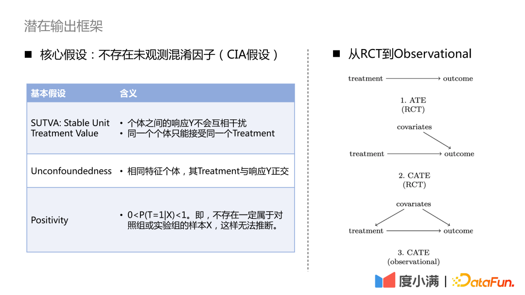
How to transition from RCT random samples to observed sample causal modeling?
For the case of RCT samples, if you want to evaluate the ATE index, you can use group subtraction or DID (difference in difference). If you want to evaluate the CATE index, you can model it through uplift. Common methods include meta-learner, double machine learning, causal forest and so on. Here we need to pay attention to the three necessary assumptions: SUTVA, Unconfoundedness and Positivity. The core assumption is that there are no unobserved confounding factors.
For the case where there are only observation samples, the causal relationship of treatment->outcome cannot be obtained directly. We need to use necessary means to cut off the backdoor path from covariates to treatment. Common approaches are instrumental variable methods and counterfactual representation learning. The instrumental variable method needs to unravel the cocoons of specific businesses and draw a causal diagram among business variables. Counterfactual representation learning relies on mature machine learning to match samples with similar covariates for causal evaluation.
02 Framework evolution of causal inference
1. From random data to observed data
Next, we will introduce the evolution of the framework of causal inference, and how it transitions to causal representation learning step by step.
Common Uplift Models are: Slearner, Tlearner, Xlearner.
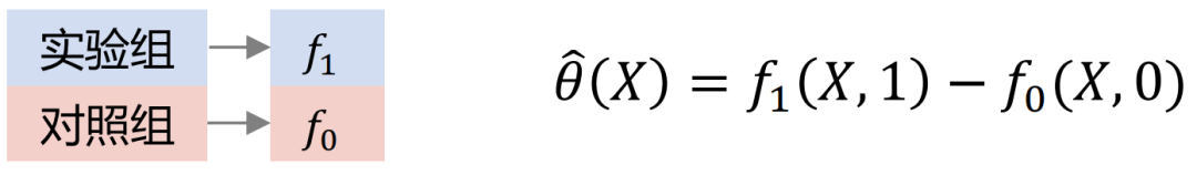
Among them, Sleaner regards the intervention variable as a one-dimensional feature. It should be noted that in common tree models, treatment is easily overwhelmed, resulting in a small estimate of treatment effect.

Tlearner discretizes the treatment, models the intervention variables in groups, builds a prediction model for each treatment, and makes a difference. It is important to note that smaller sample sizes lead to higher estimated variance.
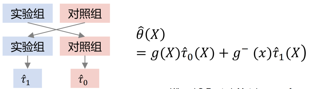
Xlearner grouped cross-modeling, and the experimental group and the control group were respectively subjected to cross-calculation training. This method combines the advantages of S/T-learner, but its disadvantage is that it introduces higher model structure errors and increases the difficulty of parameter adjustment.
Comparison of three models:
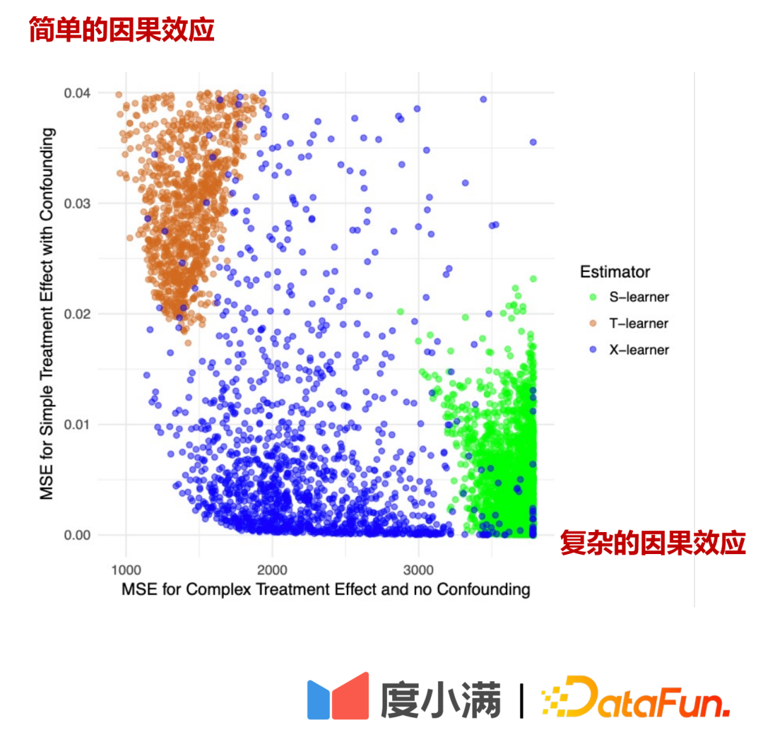
In the figure above, the horizontal axis is the complex causal effect, the estimation error of MSE, the vertical axis is the simple causal effect, and the horizontal axis and the vertical axis represent two data respectively. Green represents the error distribution of Slearner, brown represents the error distribution of Tlearner, and blue represents the error distribution of Xlearner.
Under random sample conditions, Xlearner is better for complex causal effect estimation and simple causal effect estimation; Slearner is relatively poor for complex causal effect estimation, and better for simple causal effect estimation; Tlearner is the opposite of Slearner.

If there is a random sample, the arrow from X to T can be removed. After transitioning to observational modeling, the arrow from X to T cannot be removed, and treatment and outcome will be affected by confounders at the same time. At this time, some depolarization processing can be performed. For example, the DML (Double Machine Learning) method performs two-stage modeling. In the first stage, X here is the characteristic feature of the user itself, such as age, gender, etc. Confounding variables would include, for example, historical manipulations of screening specific groups of people. In the second stage, the error of the calculation result of the previous stage is modeled, here is the estimation of CATE.
There are three ways to go from random data to observed data:
(1) Do random experiments, but the business cost is high;
(2) It is generally difficult to find instrumental variables;
(3) Assuming that all confounding factors are observed, use DML, representation learning and other methods to match similar samples.
2. Causal Representation Learning
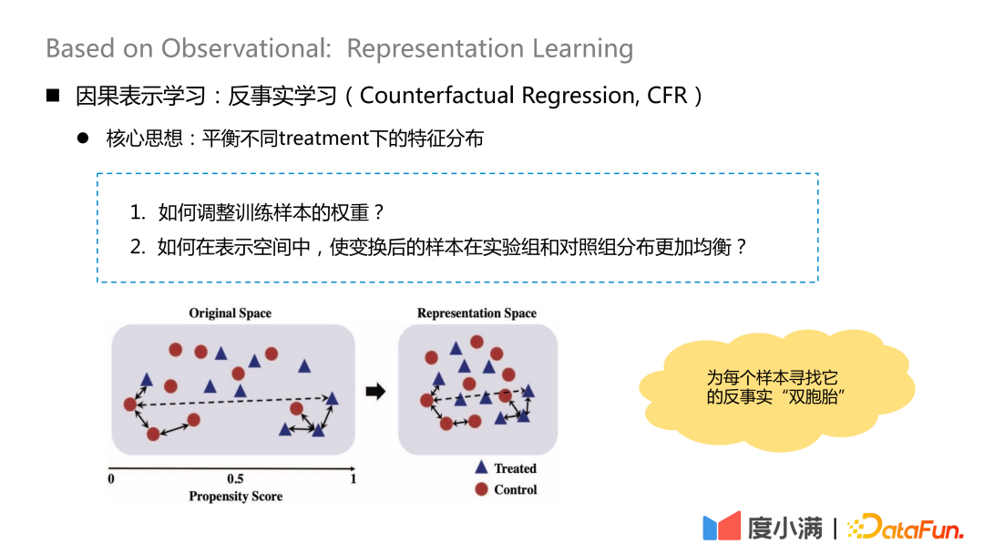
The core idea of counterfactual learning is to balance the feature distribution under different treatments.
There are two core issues:
1. How to adjust the weight of training samples?
2. How to make the distribution of transformed samples more balanced between the experimental group and the control group in the representation space?
The essential idea is to find its counterfactual "twin" for each sample after transforming the mapping. After mapping, the distribution of treatment group and control group X is relatively similar.
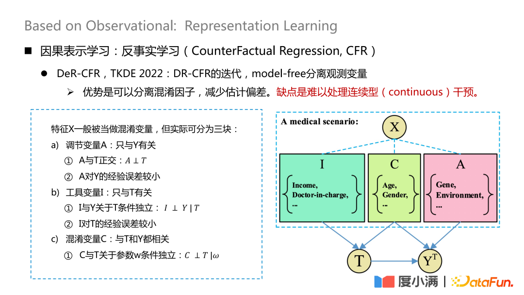
The more representative work is a paper published on TKDE 2022, which introduces some work of DeR-CFR. This part is actually an iteration of the DR-CRF model, and the model-free method is used to separate the observed variables.
Divide the X variable into three parts: moderating variable A, instrumental variable I and confounding variable C. After that, I, C, and A are used to adjust the weight of X under different treatments to achieve the purpose of causal modeling on the observed data.
The advantage of this approach is that it can separate confounding factors and reduce estimation bias. The disadvantage is that it is difficult to handle continuous interventions.
The core of this network is how to separate A/I/C variables. The adjustment variable A is only related to Y, and it needs to be guaranteed that A and T are orthogonal, and the empirical error of A to Y is small; the instrumental variable I is only related to T, and it needs to satisfy the condition that I and Y are independent of T, and the experience of I on T The error is small; the confusing variable C is related to both T and Y, and w is the weight of the network. After giving the network weight, it is necessary to ensure that C and T are conditionally independent with respect to w. The orthogonality here can be achieved by general distance formulas, such as constraints such as logloss or mse Euclidean distance.

How to deal with continuous intervention, there are also some new research papers in this area. VCNet published on ICLR2021 provides an estimation method for continuous intervention. The disadvantage is that it is difficult to directly apply to observation data (CFR scenario).
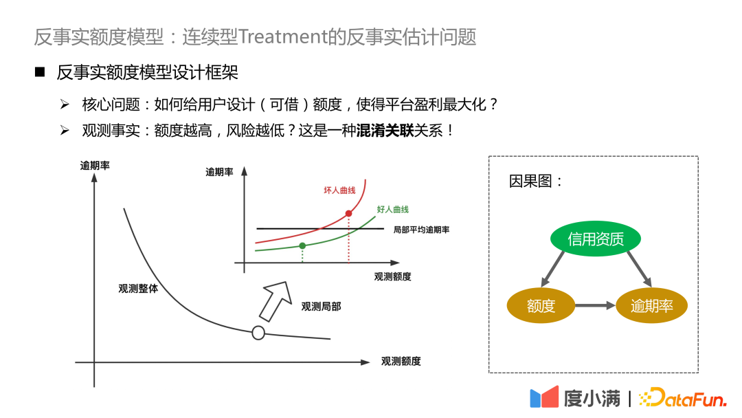
Map X to Z. Z mainly includes the I variable and C variable in the X decomposition mentioned above, that is, the variables that contribute to the treatment comparison are extracted from X. Here, the continuous treatment is divided into B segmentation/prediction heads, each continuous function is converted into a segmented linear function, and the empirical error log-loss is minimized for learning 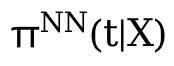 . Then use the learned Z and θ(t) to learn
  , that is, outcome. The θ(t) here is the key to handle continuous treatment. It is a variable coefficient model, but this model only deals with continuous treatment. If it is observation data, it cannot guarantee the homogeneity of each B segment data.
03 CounterfactualReal amount model Mono-CFR
Finally, let’s introduce Du Xiaoman’s counterfactual quota model, which mainly solves the problem of counterfactual estimation of continuous Treatment based on observation data.
The core question is how to design (borrowable) credits for users to maximize the platform’s profits? The prior knowledge here is that the higher the amount, the more the user borrows, and the higher the risk of default. And vice versa.
The first step is to define the profit formula. Profit = amount of income - amount of risk. The formula looks simple, but in fact there will be a lot of detailed adjustments. In this way, the problem is transformed into modeling the causal relationship between quota and risk (bad debt), quota and income on the observed data.
The second step is to estimate the user's estimated income and bad debts at each quota level, and determine the maximum profit quota.
We expect to have a profit curve as shown in the figure above for each user, and make a counterfactual estimate of the profit value at different quota levels.
If it is seen from the observation data that the higher the amount, the lower the risk, it is essentially due to the existence of confounding factors. The confounding factor in our scenario is credit qualification. People with better credit qualifications will be given a higher amount by the platform, and vice versa. The absolute risk of people with excellent credit qualifications is still significantly lower than that of people with low credit qualifications. If Latch credit qualifications, you will see that the increase in the amount will bring about an increase in risk, and the high amount has broken through the user's own solvency.
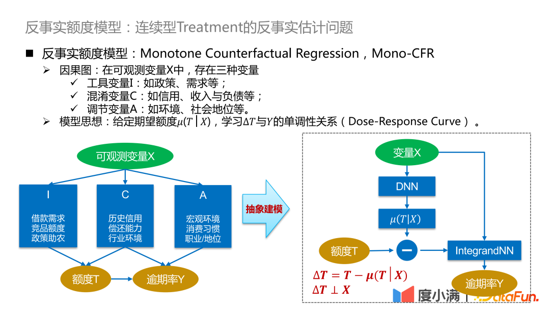
We begin by introducing the framework for counterfactual scale models. In the observable variable X, there are three variables mentioned above, most of which are confounding variables C, a small part is the adjustment variable A that is not considered by the strategy, and a part is the instrumental variable I that is only related to the intervention .
Instrumental variable I: such as policy, demand, etc., will affect the historical quota strategy, but will not affect the overdue probability;
Confounding variable C: such as credit, income, and liabilities, etc., which also affect the adjustment of the amount and the overdue probability of this person;
Adjustment variable A: such as environment, social status, etc., will affect the overdue rate.
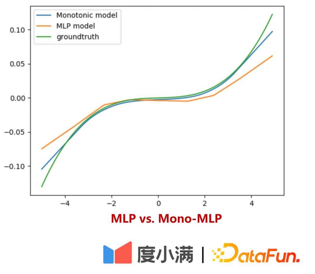
Model idea: Given the expected amount μ(T|X), learn the monotonic relationship between ∆T and Y (Dose-Response Curve). The expected amount can be understood as the continuous tendency amount learned by the model, so that the relationship between the confounding variable C and the amount T can be disconnected, and converted into a causal relationship learning between ∆T and Y, so as to compare the distribution of Y under ∆T good characterization.
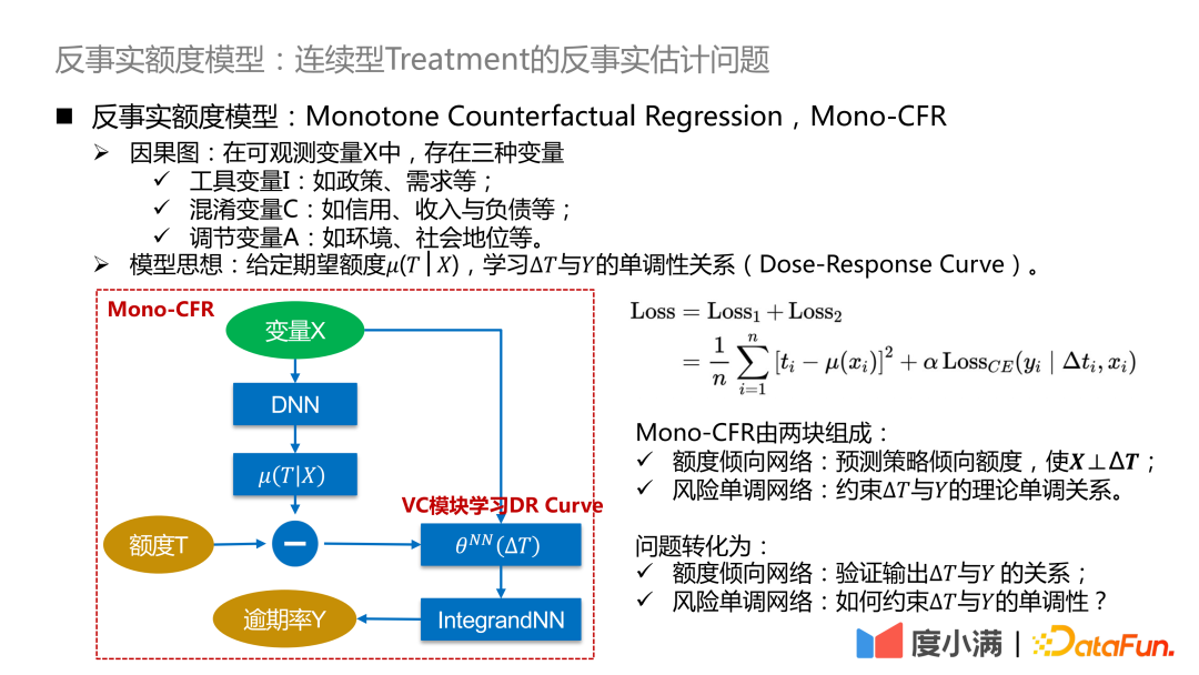
Here we further refine the above abstract framework: convert ∆T into a variable coefficient model, and then connect to the IntegrandNN network, the training error is divided into two parts:
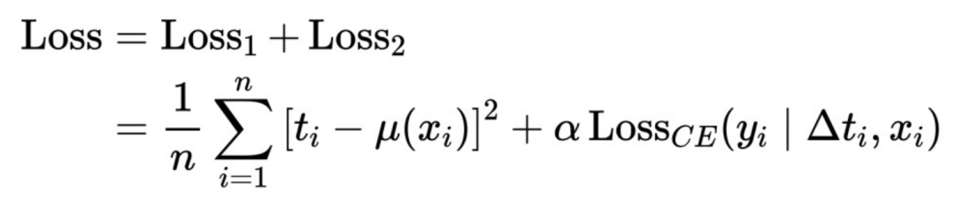
Here α is a hyperparameter that measures the importance of risk.
Mono-CFR consists of two parts:
Quota propensity network: prediction strategy tends to quota, so that X⊥∆T;
Function 1: Distill out the most relevant variables in X and T to minimize the empirical error;
Function 2: Anchoring approximate samples on historical strategies.
Risky Monotonic Networks: Constraining the theoretical monotonic relationship between ∆T and Y.
Function 1: impose independent monotone constraints on weak coefficient variables;
Function 2: Reduce estimation bias.
The problem turns into:
Quota propensity network: verify the relationship between the output ∆T and Y;
Risky Monotonic Networks: How to constrain the monotonicity of ∆T and Y?
The actual quota tendency network input is as follows:
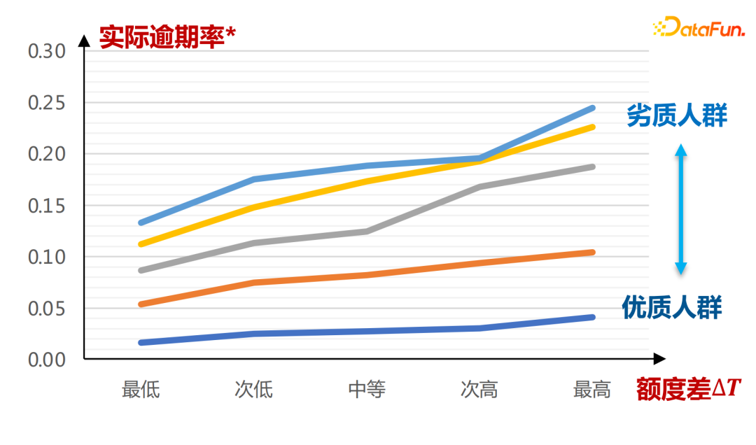
The horizontal axis is the group of people defined by the A card score. It can be seen that under different tendencies of the amount μ(T|X), the amount difference ∆T and the overdue rate Y present a monotonically increasing relationship. The steeper the change curve of the actual overdue rate is, the steeper the slope of the entire curve will be. The conclusions here are drawn entirely through historical data learning.
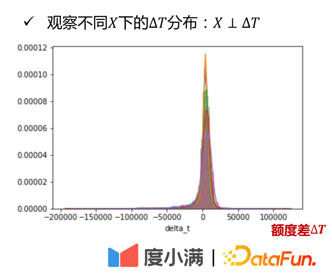
It can be seen from the X and ∆T distribution diagrams that the credit difference ∆T of different qualified groups (distinguished by different colors in the figure) is evenly distributed in similar intervals, which is explained from a practical point of view  . From a theoretical point of view, it can also be strictly proved.
The second part is the implementation of the risky monotonic network:
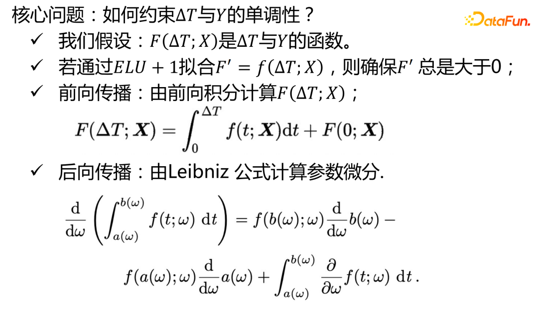
The mathematical expression of the ELU+1 function here is:
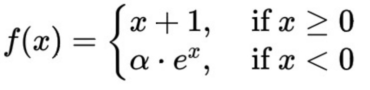
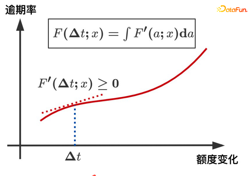
∆T and the overdue rate show a monotonically increasing trend, which is guaranteed by the fact that the derivative of the ELU+1 function is always greater than or equal to 0.
Next, show how the risk monotonic network is more accurate for weak coefficient variables:
Suppose there is such a formula:

It can be seen that x1 here is a weak coefficient variable. When the monotonic constraint is imposed on x1, the estimation of the response Y is more accurate. Without such a separate constraint, the importance of x1 would be overwhelmed by x2, leading to increased bias in the model.
How to evaluate the risk estimation curve of the quota offline?
Divided into two parts:
Part 1: Explainable Verification
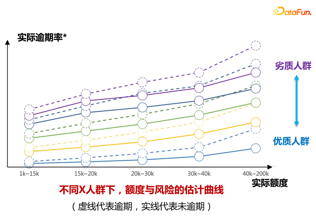
Under different qualification groups, draw the quota risk change curve as shown in the figure above, and the model can learn the distinction between the actual quota and overdue rate of different gears for different qualification groups (identified by different colors in the figure).
The second part: use the small flow experiment to verify that the risk deviation under different amount increase ranges can be obtained through uplift binning.
Conclusion of the online experiment:
Under the condition of a 30% increase in the quota, the user's overdue amount will decrease by more than 20%, the loan will increase by 30%, and the profitability will increase by more than 30%.
Future model expectations:
A clearer separation of instrumental variables and moderator variables in a model-free form makes the risk transfer performance of the model better on poor-quality populations.
In actual business scenarios, Du Xiaoman's model evolution iteration process is as follows:
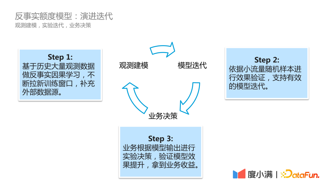
The first step is observation modeling, continuously scrolling historical observation data, doing counterfactual causal learning, constantly opening new training windows, and supplementing external data sources;
The second step is model iteration, which verifies the effect based on small flow random samples and supports effective model iteration;
The third step is business decision-making. The business makes experimental decisions based on the model output, verifies the improvement of the model effect, and obtains business benefits.
The above is the content of this sharing, thank you!
Editor: Huang Jiyan
