Causation, causal inference, what is causation?

What is causality?

When we ask "why", what are we asking?

Shallow men believe in luck or in circumstance. Strong men believe in cause and effect. ― Ralph Waldo Emerson

Chapter 1 - Preface : Introduce the discussion background of the question "What is causality?" in plain language, and summarize several traditional philosophical views, and the existence of these traditional definitions compared with the statistical causal model below defect.
Chapter 2 - Event Causation
2.1. Randomized controlled trials
2.2. Causal view of interventionism
2.3. Virtual reality model (RCM)
2.4. Bayesian Networks
2.5. Structural Equation (SEM) + Structural Causal Model (SCM)
2.6. Counterfactual Reasoning in SCM
Chapter 3 - Process Causality : Causal Loop Diagrams (CLDs) and Differential Equations
Chapter Four - Epilogue

In addition to the preface, the rest of this article assumes that readers have understood basic probability theory (probability, conditional probability, Bayes theorem, random variables, expected values, independent events), basic graph theory (nodes, edges, directed acyclic graphs), Basic knowledge of probability graphical models (Bayesian network, d-separation), statistical basis (randomized controlled trials), etc.

In addition, this article can be regarded as an introduction to Judea Pearl's "Causality".

Reference system: Guanhe causal analysis system

Reprinting of the full text is prohibited, please indicate the source and send a private message for large-scale citations.

I. Introduction

Cause and effect are everywhere in life. Economics, law, medicine, physics, statistics, philosophy, religion and many other disciplines are inseparable from causal analysis. However, causality is very difficult to define compared to other concepts such as statistical correlation .

Using intuition, we can easily judge the causal relationship in daily life; however, it is often beyond the scope of ordinary people to accurately answer the question "what is causal relationship?" in clear and unambiguous language.

(Interested readers may wish to pause reading, and then try to give a definition of "causality".)

It has to be admitted that answering this question is very difficult, so that some philosophers believe that causality is irreducible, the most basic cognitive axiom, and cannot be described in other ways. However, the many statistical causal models that will be described in this paper will be a powerful rebuttal to this view.

On CSDN, there are also some discussions on causality. Unfortunately, most of the answers to this question focus on epistemology, that is, "how to respond to Hume's induction problem?" and "we How do you know that the causal relationship we recognize is reliable?" Everyone seems to agree that "what is causal relationship" is a premise that is too trivial to discuss (but it is obviously not the case), and they fall into skepticism and transcendentalism, so they cannot give Develop a practical causal model . In fact, causality is an ontological topic : we need to find an intuitive, broad enough, but specific enough definition to describe causality; on this basis, we also need a set of reliable methods for determining causality .

Commonly used statistical causal models all adopt the interpretation of interventionism : the definition of causal relationship depends on the concept of "intervention" ; external intervention is the cause, and the change of the phenomenon is the effect .

Before doing that, let's take a look at other traditional definitions of "causality" and why they are not intuitive.

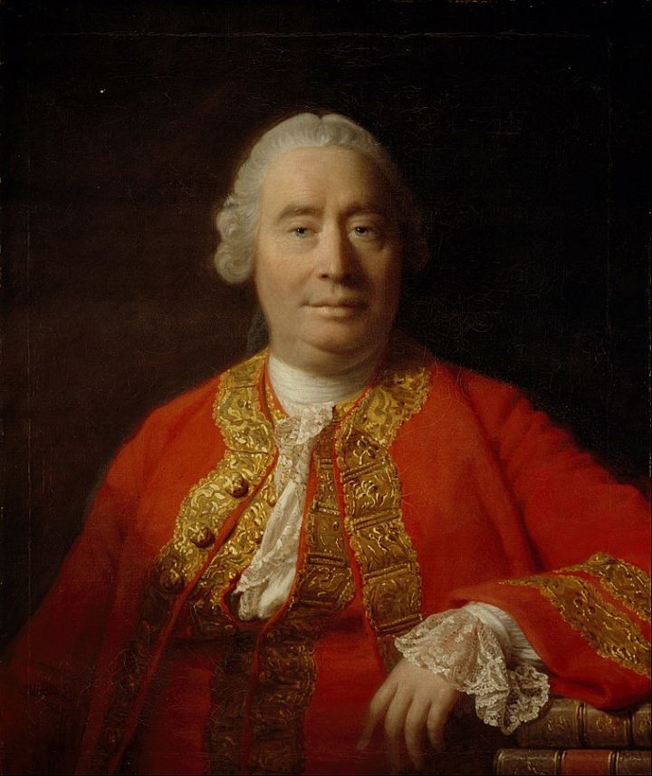
David Hume

Hume: Causation is " constant conjunction ." If we observe that A always precedes B, and that events A and B are always connected, then A causes B, or A is the cause of B.

Rebuttal: Let A denote the rooster crowing, and let B denote the sunrise. Under natural conditions, there is always a rooster crowing before sunrise, but no one thinks that the rooster crowing causes the sunrise. If we intervene and imprison all the roosters so that they cannot crow, the sun will still rise as usual.

Here, it is necessary to pay attention to a detail:

David Hume (1711-1776).

Karl Pearson (1857-1936).

Pearson, who proposed the concept of "statistical correlation", was born more than a hundred years later than Hume.

Our current way of thinking has not existed since ancient times: the common sense that we take for granted may never have appeared in the minds of the ancients.

Before statistics became a serious discipline and Pearson made a clear separation between correlation and causation, most people conflated correlation and causation. Even now, there are not a few people who think that correlation means causation.

We don't need to regard Hume's definition as a golden rule because of his historical status. Therefore, the frequent connection used by Hume can only define correlation, not causation.

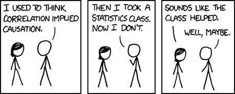
Correlation does not necessarily imply causation

Correlation does not imply causation.

Correlation is symmetric, while causation is asymmetric. If A is the cause of B, then B is the effect of A, but we would never simultaneously say "event A is the cause of event B, and event A is the effect of event B". As for correlation, the correlation between random variables X and Y is defined as corr(X,Y)=cov(X,Y)σXσY=E[(X−μX)(Y−μY)]σXσY, so there must be corr (X,Y)=corr(Y,X) .

The asymmetry of causality has been used to refute Hempel's use of the DN model to define "scientific explanation", but this is a digression belonging to the philosophy of science.

The above two intuitions can refute the following series of causal definitions that do not use the concept of "intervention".

Sufficient cause: A→B

Necessary cause: A←B

Naive counterfactual causality: (A→B)∧(¬A→¬B)

Add probability theory and use correlation to define causality.

A typical counterexample: use event A to represent "increased sales of ice cream", and use event B to represent "increased number of drowning deaths". There is a positive correlation between A and B, but we all know that there is no causal relationship between A and B. They are all caused by a common factor "summer". It can be seen that only using the tools of probability and statistics is not enough for us to make rational causal inferences in reality .

INUS条件：原因是Insufficient but Necessary parts of a condition which is itself Unnecessary but Sufficient。

Examples of INUS conditions, but not causes, are not hard to construct: Lightning, haystacks, firefighter negligence, and dry air are all INUS conditions for a fire. However, we know that lightning and thunder always meet the "if there is lightning, then there must be thunder"; therefore, thunder is also the INUS condition of fire, but it is not the cause of fire.

The above-mentioned series of models/definitions all have a common flaw: given a causal relationship, these models can be applied perfectly; however, given such a model, we cannot directly determine the causal relationship between different variables, because A single model can simultaneously describe many different causal and even non-causal relationships .

Philosophers do not seem to have come up with a satisfactory account of causality. But this is at best a misconception popular among lovers of philosophy. Ordinary philosophy lovers usually do not know more about causality than Hume and Kant, and it is extremely rare to know Lewis, inevitability, and pluralism. In fact, in statistics, economics and other fields, there are already a large number of mature and put into use causal models, which accurately reflect our intuitive understanding of causality and can be described by precise mathematical language.

2. Event causation

When we say "A is the cause and B is the corresponding effect", what "things" can A and B be?

In general, we think of A and B as some kind of event , and that A must happen before B. Because "cause" must happen before "effect", if A causes B, then it is impossible for B to cause A at the same time—two events cannot be mutually causal . It can be seen that there is an asymmetry in the causal relationship .

Philosophers have had a lot of discussions ( Backward Causation ) on the condition that "in time, the cause must precede the effect" , many of which involve cutting-edge quantum mechanics. However, we still have no reason to abandon this condition. Because different models have different scopes of application, and the scope of application of causal models is mainly macroscopic phenomena, economics, medical treatment, and complex power/circuit systems. Regardless of the conclusions of microphysics, its validity in known fields is not affected. Influence.

Some people may question, why can't two things cause and effect each other? For example, let A1 denote the number of sheep on the prairie, and let B1 denote the number of wolves on the prairie; ceteris paribus, an increase in wolves will lead to a decrease in sheep, a decrease in sheep will cause a decrease in wolves, and a decrease in wolves will in turn lead to a decrease in sheep. The increase of sheep leads to the increase of wolves; A1 and B1 are mutually causal.

It is worth noting that A1 and B1 represent a certain process , rather than an event at some fixed time point , so the complete causal relationship between A1 and B1 cannot be expressed by event causality. So, for this question, I have the following responses:

We can split A and B at each time point into separate events in chronological order, that is, B1 (wolves increase) → A1 (sheep decrease) → B2 (wolves decrease) → A2 (sheep increase). In this way, event causality can also express the relationship between A and B.

For procedural causality, we have another model—causal loop diagram (CLD), which will be introduced in Chapter 3 of this paper.

Process causation is more complex than event causation. Before understanding the process causal model, we need to understand the simpler event causal model.

For event causality, the most mature and extensive model is the Structural Causal Model (hereinafter referred to as SCM) . SCM combines structural equations (SEM), virtual reality models (RCM), probabilistic graphical models (mainly Bayesian networks), and applies them to causal analysis. All kinds of commonly used causal models can be regarded as subcategories of SCM. Next, I will give a detailed introduction to RCM, Bayesian network, and SEM in the order of the development of SCM.

2.1. Randomized controlled trials

As any introductory statistics textbook will mention, statistical models based on observations cannot reliably identify causal relationships. To determine causality, a randomized controlled trial (Randomized Controlled Trial) must be passed.

In a simple randomized controlled trial, test subjects (usually volunteers participating in the research, each subject is represented by u below) will be randomly divided into two groups: the treatment group (treatment group, represented by t below) and the control group ( control group, denoted by c below).

We have different randomization methods such as simple randomization , randomized block design , paired design . When using a random block design, the researcher will first divide individuals into different blocks according to their characteristics (age, gender, etc.), and then implement simple random grouping within each block. When using a paired design, the researcher will pair individuals who are very similar in all aspects (such as twins, the same person at different time points), and randomly select one individual from each pair as the experimental group and the other as the control group .

Subjects in the experimental group will receive the intervention, but subjects in the control group will not receive any intervention/intervention. In medical experiments, subjects in the experimental group receive the real treatment, while those in the control group receive only a placebo. After the experiment is over, the researchers compare the results of the experimental and control groups.

If we denote our outcome variable of interest by Y, then we can denote the outcome of a randomized controlled trial with the following notation:

Yc(u) is the outcome variable Y exhibited by subject u under the control condition.

Yt(u) is the outcome variable Y exhibited by subject u under the condition of the experimental group.

In research, we usually ask whether Yt(u) is statistically significantly different from Yc(u). This process involves more specific statistical hypothesis testing, which has nothing to do with the main content of this article. However, we can at least realize that the difference between t and c is the "cause" in the causal relationship, and the difference between Yt(u) and Yc(u) is the "effect" in the causal relationship .

2.2. Causal view of interventionism

Based on the basic framework of randomized controlled trials, we can establish an interventionist view of causality.

An interventionist causal model consists of three parts:

All systems U : A set containing all systems u. A system u The object we are discussing can be a human body, a machine, a planet, a chemical reaction system, an economic entity, etc.

All interventions T : A set containing all possible interventions t. For example, suppose the system U in question is a black box with two buttons, one red and the other green, then all possible interventions are {press the red button, press the green button, both buttons are Press, neither button press }. (In this specific example, depending on the structure of the black box, there may be more than four possible intervention methods, so this is just a simplified model for intuitive understanding.)

State function Y : Input a system u and an intervention method t, and output a certain state y of the system, written as y=Yt(u). For example, in a medical experiment, Y could reflect "u (patient A)'s y (blood pressure) after intervention t (taking blood pressure medication)". Note that y does not have to completely describe all parts of the state of u, it is also possible to reflect only a few variables . Of course, we can let y represent the motion state of all the molecules in a patient's body, but this kind of overly complicated state function is often of little practical value. However, in a system such as a simple circuit, it is not only feasible but also advantageous to fully express the state of each node of the circuit. Therefore, when establishing a causal model, we need to analyze specific issues and choose an appropriate state function.

It is worth noting that since the definition of "result" involves the difference between Yt(u) and Yc(u), and a single intervention only explains t but not c, T must contain an expression indicating "non-intervention" . Intervention method c . That is, in a causal model, any system must have a "natural state" without intervention . If the actual situation is too complicated and it is difficult to find a natural state without intervention, we can set a certain intervention method c as "non-intervention" by default .

therefore:

Any causal model of interventionism must clearly point out a way of intervention that represents "non-intervention".

When we ask "why does phenomenon y1 occur?", we are actually asking: "In my causal model of the world, the phenomenon in the state of nature is y0=Yc(u), but I observe phenomenon y1≠y0 .So I think what actually happens is that y1=Yt(u) where t≠c. What is the difference between t and c?"

Or, to put it more simply, when we ask "Why A", we tend to omit the second half of the sentence: "Why A, not B?"

Taking the first few results of Zhihu’s search for “why” as an example, we can find that the “default state” way of thinking is indeed ubiquitous.

Example 1: Why don't boys chase girls nowadays?

Default state: Boys should chase girls.

Example 2: Why would someone order cat poop coffee worth more than 200 yuan a cup?

Default state: Most people will not spend more than two hundred yuan for a cup of coffee.

In other cases, the two interlocutors may choose different default states, resulting in the following dialogue:

A: "Why did you do A?"

B: "Why not?" (By default, "doing A" is a natural state, shifting the responsibility of the argument to A)

In the next section (2.3), we will develop this set of intuitions into a formal virtual fact model.

However, I would like to make some clarifications on Granger causality . Definition of Granger causality: A is said to be Granger-causal to B if knowing the occurrence of event A helps to predict subsequent event B. However, Granger causality only includes observation, but not intervention . Direct manipulation of A does not necessarily affect B, which is inconsistent with our daily intuition of causality. Therefore, although Granger causality is called "cause and effect", it is only a concept of statistical correlation, not a real concept of causality. In what follows, I will not discuss Granger causality further.

2.3. Virtual reality model

2.3.1 The Rubin Causal Model (RCM) was proposed by Donald Rubin. In RCM, the causality "effect" is defined as δ(u)=Yt(u)−Yc(u).

In real life, we often consider more than one system—for a drug under development, what we are most interested in is undoubtedly its effect on all target groups , not just a certain patient A. Continuing to use RCM’s definition of causality, then the “effect” of an intervention “cause” on all individuals in the group is E[δ(u)]=E[Yt(u)−Yc(u)]=E[Yt(u )]−E[Yc(u)]. (obtainable from the linearity of the expected value)

From the perspective of God, the above definition is not complicated. Even though the variable y=Yt(u) is not a numeric variable, we can define δ(u) in other ways. From a broader perspective, the subtraction in the RCM definition is not necessarily the subtraction of the real number field; for more complex variables y (such as tensors, probability distributions), we can use other subtractions, as long as they meet the mathematical specifications and specific research needs. Can.

But in real life, we cannot get perfect information:

It is not possible to know Yc(u) and Yt(u) at the same time . Since each person is unique and each time node is also unique, after receiving an intervention and showing a new state, it is impossible for the system to perfectly restore to its original state and accept another intervention. This situation is called " the Fundamental Problem of Causal Inference" (hereinafter referred to as FPCI ).

It is impossible to know the situation of each individual at the same time. Just as when testing the quality of mobile phones under extreme conditions, it is impossible for us to smash every mobile phone. We can only randomly draw samples from the group, and then use the statistical data of the samples to infer group parameters.

The problem of "unable to know every individual at the same time" has been solved by conventional statistical methods. But to avoid FPCI, we must make additional assumptions about the distribution of population parameters, including but not limited to one or more of the following:

Stable unit treatment value assumption (SUTVA for short): The intervention of any individual u1 will not affect the state of another arbitrary individual u2. SUTVA allows us to treat the responses of each individual in the sample as an independent event, thereby reducing the sample size, model size, and modeling time we need.

Assumption of constant effect : The effect of an intervention is the same for all individuals. For example, the effect of a certain antihypertensive drug on everyone is to lower blood pressure, and will not increase blood pressure—even if there is, it is just statistical noise, which can be resolved with large samples, the theorem of large numbers, and the central limit theorem . Then, we can get δ^(u)=Yt¯(u)−Yc¯(u), and use the average effect within the sample to estimate the causal effect of this intervention on all individuals.

Assumption of homogeneity : For any individual u1 and u2, and any intervention t∗, there is always Yt∗(u1)=Yt∗(u2) . The homogeneity assumption is stronger than the same effects assumption. For example, a simple FizzBuzz computer program should behave exactly the same at different points in time. Although at the same point in time, we cannot test its output under different inputs at the same time, but its performance at different points in time must be the same. If we regard "FizzBuzz programs at different time points" as a group, then the individual "FizzBuzz programs at each time point" all meet the homogeneity assumption.

2.3.2 Insufficiency of virtual reality model

Although RCM provides a causal model that can be defined mathematically and statistically, its shortcomings are also obvious: when intervening, we usually can only change one variable at a time , and the observed state has only one variable. If we increase the variables, the size of the model, the training data required, and the training time will all increase exponentially . In the next section, we can see that the conditional independence information of the Bayesian network prior can alleviate this difficulty.

In addition, the structure of RCM from the "cause" of the independent variable to the "effect" of the dependent variable is almost completely a black box , lacking clearer interpretability. Therefore, the problems that a single RCM can solve are relatively limited. In contrast, structural causal models can provide more detailed explanations for causal laws, causal relationships among multiple variables.

2.4. Bayesian Networks

Bayesian network is a probabilistic graphical model based on directed acyclic graph (DAG for short) . Although the Bayesian network cannot directly represent causality, it can only represent correlation, but its graph structure is the basis of SCM.

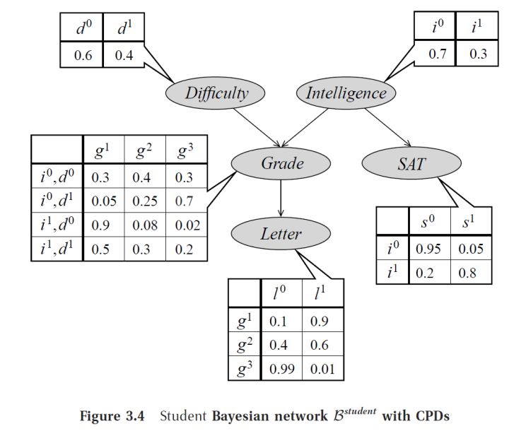
Bayesian Network Example

In a Bayesian network, each node is a random variable that represents an event. Usually, this random variable follows some discrete or continuous distribution. A node X stores the distribution of X given all its parent nodes pa(X), that is, P(X=x|pa(x)). pa(X) means all parent nodes of node X, that is, all nodes that "have directed edges directly pointing to X". Take the above picture as an example, pa(Grade)={Difficulty,Intelligence} .

Compared with the original joint distribution model, the Bayesian network (and all other probabilistic graphical models) has the biggest advantage of increasing the prior information of the conditional independence between the variables, thereby reducing the size of the model and inferring with the model , Study time . For example, there are 5 variables in the figure above. If the naive joint distribution model is used to model the conditional probability table, the volume of the conditional probability table will be 2×3×2×2×2=48. After using the Bayesian network, the conditional probability table The total volume of is 2+2+4×2+2×1+3×1=17. In a small network, the effect of this simplification is not obvious, but in a large network, assuming that each variable has a value, the volume of the joint distribution model will be O(an), and a suitable Bayesian The Si network may be able to reduce the volume complexity to the polynomial level. The most extreme case is Naive Bayes, that is, all random variables are independent, and the volume complexity of the model is O(an).

Conditionally independent information is a priori, and they are often provided by task-related experts rather than learned from data. This approach can ensure the reliability of the network structure. (The discussion here is parameter learning rather than structure learning. The network structure is known but the parameters are unknown; for the latter, we have the Chow-Liu algorithm, but it is not discussed here.) Later, we will also find that a similar prior Causal assumptions play an important role in SCM.

2.4.1. d-separation

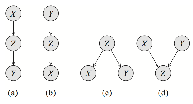
As shown in the figure, for three nodes/variables in a Bayesian network, there are three basic structures. Two different conditional independence assumptions. Use X⊥Y to denote independence between X and Y:

cascade : A→B→C , then there must be (A⊥C)|B and A⊥̸C .

common parent : A←B→C, also (A⊥C)|B and A⊥̸C .

V-structure : A→B←C , there must be A⊥C and (A⊥̸C)|B , which is different from the conditional independence of the first two basic structures.

In order to answer the question "Given a set Z of random variables, whether the random variables A and B are conditionally independent", we need to introduce the concept of d-separation. The full name of d-separation is "directed separation".

A set of nodes O can separate nodes A and B by d if and only if: Given O, there is no active path between A and B.

For an undirected and acyclic path P between A and B, if every three consecutive nodes on P meet one of the following four conditions, then P is a valid path:

X←Y←Z and Y∉O

X→Y→Z and Y∉O

X←Y→Z and Y∉O

X→Y←Z and Y∈O. This situation is known as Berkson's Paradox : When the common outcome of two independent events is observed, the two independent events are no longer independent of each other. For example, if two coins are tossed, the upside of coin A and the upside of coin B should be independent of each other; The faces are no longer independent of each other.

Correspondingly, if, given O, a path P is not a valid path , then we say that the set of O nodes d separates the path P. The notion of a d-separation applies to two nodes, and also to a path between two nodes, the latter being useful in the definition of the "backdoor criterion".

If two variables are not separated by d, the state between them is called a d-connection .

The d-separation can greatly simplify the judgment of conditional independence such as (X⊥Y)|Z in the Bayesian network. Pearl generalized it further and proposed the concept of graphoid . A graphoid is a set of statements in the form of "knowing variable Z, then variable X and variable Y are independent of each other", obeying the following five graphoid axioms :

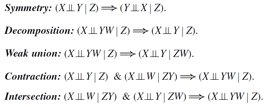
Remarks on the Chinese translation of graphoid: There is no authoritative Chinese translation of graphoid yet, and there are hardly any related Chinese materials on the Internet. When I chose the translation name, I referred to the translation of matroid. Since matrix is a matrix and matroid is a matroid, then graph is a graph, so graphoid should be called a quasi-graph.

The concept of mimesis appears only in Pearl's writings. However, if we adopt the definition of "independent events" in probability theory, then we can deduce them as theorems. It can be seen that the "independence" of probability theory conforms to the axiom system of the drawing. Of course, the establishment of intersection requires an additional condition: for all events A, if A≠∅, then P(A)>0.

2.4.2. Why are Bayesian networks not suitable for causal modeling?

After having a learned Bayesian network, we can use it for various inferences, mainly probabilistic inference P(Xi|Xj1,Xj2,Xj3,...,Xjk): known Xj1,Xj2,Xj3, ..., Xjk and other random variables, find the conditional probability of another random variable Xi. The superiority of Bayesian networks is reflected in the fact that even with a large number of missing, unknown variable values, it can use marginalization operations to perform probabilistic inferences without hindrance . In SCM, this function still has a very important position.

If we think of the arrows as going from cause to effect, and A→B as A causing B, then Bayesian networks seem to be able to express causality. However, Bayesian networks by themselves cannot distinguish the direction of causality . For example, the causal direction of A←B←C is completely opposite to A→B→C, but under the model description of Bayesian network, the probability distribution and conditional independence assumption expressed by them are exactly the same.

In addition, the "given/known" in the probability theory "given/known random variable Z" can only be used to express observation, not intervention . For example, the probability values of P(raining|ground is wet) and P(ground is wet|raining) are both high, where "given "the ground is wet"" and "given "raining"" It is all the result of observation rather than intervention . Use do(X) to mean "intervention, making event X happen" , and now consider another situation: P(rain|do(the ground is wet)). Intuitively, it is obvious that P(rain|do(the ground is wet)) < P(rain|the ground is wet), because wetting the ground does not cause rain.

In summary, Bayesian networks, while powerful, cannot accurately describe causal relationships. The following SEM will mainly solve this problem. In the process of learning Bayesian networks, we should also try to avoid using words related to "cause and effect"-in Bayesian networks, A→B does not necessarily mean that A leads to B.

2.5. Structural equation + structural causal model

To represent causal relationships, we need to refine Bayesian networks. Structural Equation Model (SEM) is very commonly used in the fields of economics and engineering. After adding the components of SEM on the basis of Bayesian network, we are one step closer to a perfect SCM (Structural Causal Model).

2.5.1. Symmetry breaking

In a Bayesian network, the probability distribution P(X=x|pa(X)) of a node X is determined by its parent node pa(x), recorded in a conditional probability table. However, conditional probability tables and some simple continuous probability distributions are invertible . For example, for random variables X and Y, if Y=αX+β, then we can manipulate the algebraic expression to get X=Y−βα. However, this symmetry is counterintuitive in causality . Symmetrical algebraic expressions show that if we change Y, X will change accordingly; however, modifying the reading of a thermometer does not change the ambient temperature, and adjusting the hour hand of an alarm clock does not change the true flow of time.

Thus, in SEM, we represent some variable X with a functional equation: X=fX(pa(X),u(X)) . Among them, pa(X) represents the endogenous variable (endogenous variable) in the parent node of X ; u(X) represents the exogenous variable (exogenous variable) in the parent node of X , and there is only one. Endogenous variables depend on other variables, expressed in SCM as "a node with a parent node", that is, at least one edge points to the node; exogenous variables are independent of other variables, expressed in SCM as "a node without a parent node ”, that is, no edge points to this node.

In traditional path analysis research, fX is usually a linear function, and the definition of causality is also limited to α in Y=αX+β. However, now that the data is becoming more and more complex, we can completely use nonlinear functions and non-parametric models. Correspondingly, the definition of "cause and effect" has also changed from the path parameter α to a broader "change transmission" , see the previous part of RCM. As a broad modeling framework, SCM can generate a wide variety of complex models.

Under the broadest conditions, the function fX is not invertible. We need to understand X=fX(pa(X),u(X)) as "(nature/model itself) assignment to X" , not just an ordinary algebraic equation. SCM requires that all arrows A→B must mean "A directly leads to B". Therefore, in the process of causal inference, we must reason in the direction of the causal arrow, and the order cannot be reversed.

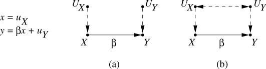
Figure 1: Schematic diagram of a structural causal model

As shown in the figure above, UX and UY are exogenous variables, X and Y are endogenous variables, and X can lead to Y. In graph (a), there is no edge connecting UX and UY, while in graph (b), there is a two-way arrow between UX and UY represented by a dotted line. In SCM, we use a one-way arrow to express a direct causal relationship , and a two-way arrow to indicate that there may be unknown confounding variables between two exogenous variables .

Exogenous variables such as UX and UY can represent "environmental noise not accounted for in the model", thereby adding a stochastic element to seemingly non-random structural equation models . Therefore, SEM is not completely certain, and it can also have characteristics such as probability and uncertainty; SCM is broader than ordinary Bayesian networks. In addition, an SCM describes the generation principle of the data, not just the probability distribution observed on the surface, so the SCM is more stable than the Bayesian network.

2.5.2. Intervention

As mentioned above, SCM is a generalization of Bayesian network. A general Bayesian network can answer two types of problems:

Conditional probability: P(Y|E=e) , where Y is the set of unknown variables we are interested in, E is the set of known variables we observe , and e is the value of E we observe . E can be the empty set, which means "we did not observe any variable".

Maximum Posteriori Probability (MAP): arg⁡maxyP(Y=y|E=e) , what we want to find is a set of most likely Y values.

If the complexity of the algorithm is not considered, a model that can estimate the conditional probability must be able to estimate the MAP, so the following will only discuss the case of the conditional probability.

On the basis of "observation", SCM can also achieve "intervention" : P(Y|E=e,do(X=x)). In it, we intervene in the system to force a set of variables X to have the value x. In the case where X is an empty set, SCM is not much different from ordinary Bayesian networks.

Take the following figure as an example, and I will show how SCM achieves intervention.

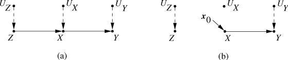
Figure 2: An SCM

In this SCM, the relationship among variables X, Y, Z can be expressed by the following structural equation:

Z=fZ(UZ)

X=fX(Z,UX)

Y=fY(X,UY)

In this model, we assume that the three exogenous variables UX and UY are independent from UZ. Therefore, there is no edge connection between UX and UY and UZ in graph (a) and graph (b).

As shown in Figure (b), when we intervene do(X=x0) , we cut off all edges pointing to X and assign X to x0 . Thus, the new SCM includes a new set of structural equations:

Z=fZ(UZ)

X=x0

Y=fY(X,UY)

To sum up, an SCM (written as M1 ) estimates PM1(Y|E=e, do(X=x)) in the following way: after completing the intervention of do(X=x) in the original model M1, a new The model M2 . Subsequently, PM2(Y|E=e) is estimated on M2.

Some people may ask: "Is there any essential difference between observation and intervention?"

An everyday example answer is as follows:

Let A represent "environmental temperature", and B represent "thermometer reading", and the causal relationship between A and B is A→B. By default, the thermometer is immune to external intervention. Therefore, observing an increase in the thermometer reading, we can deduce that the ambient temperature has increased. However, when we intervene directly with the thermometer (for example, hold the thermometer with our hands), we intervene do (B=b1), so that the reading of the thermometer becomes b1; at the same time, because it is intervention rather than observation, from A to B The causal arrow is cut off and we have A↛B or A B .

Assuming that b1 is a higher temperature, then P(A=b1|B=b1) represents "the probability that the actual ambient temperature is b1 when the reading of the thermometer is observed to be b1 in the natural state"; P(A= b1|do(B=b1)) represents "the probability that the actual ambient temperature is b1 when external intervention makes the thermometer read b1". Obviously, P(A=b1|B=b1)>P(A=b1|do(B=b1)), it can be seen that observation and intervention are two completely different behaviors. Observations do not affect the natural state of the model, but interventions do.

2.5.3. Mathematical principles of causal inference

In this section, I present the mathematical basis of SCM for causal inference.

We say that an SCM has the Markov property if and only if the SCM does not contain any directed cycles, and all exogenous variables are independent of each other . Because exogenous variables are usually understood as some kind of "error term" or "noise term", if there is a correlation between some exogenous variables, there may be confounding variables between them . In a Markovian SCM, we can get the following fundamental theorem:

Causal Markov condition : P(v1,v2,...,vn)=∏i=1nP(vi|pa(vi))

Among them, vi represents the variable we are interested in, and pa(vi) represents all endogenous variables in its parent node. Using causal Markov conditions, we can decompose a joint probability distribution into the product of multiple conditional probability distributions.

An SCM that meets the causal Markov condition still meets the causal Markov condition after intervention, and the conditional probability is calculated as follows:

P(v1,v2,...,vn|do(X=x))=∏i=1,vi∉XnP(vi|pa(vi))|X=x

Among them, X is a series of variables subject to intervention, and x is the value of the variable in X after the intervention. P(vi|pa(vi))|X=x means that the variable in pa(vi) is also in X (that is, in pa(vi)∪X) will be assigned the corresponding value of x.

figure 2

Taking Figure 2 as an example, before the intervention, P(Z,Y,X)=P(Z)P(X|Z)P(Y|X) , and after the intervention do(X=x1), P(Z ,Y|do(X=x1))=P(Z)P(Y|X=x1) . Note that since the causal arrow from Z to X has been cut, P(Z)=P(Z|do(X=x1)) , since changing X directly cannot affect Z.

In "Causality," Pearl demonstrates a broader conclusion:

P(Y=y|do(X=x))=∑tP(Y=y|T=t,X=x)P(T=t)

Among them, each t represents a possible value of all parent nodes of X. Since all arrows pointing directly to X have been cut off, it is natural to have P(T=t|X=x)=P(T=t) .

2.5.4. Back-door criterion

Consider the SCM shown in Figure 3 below:

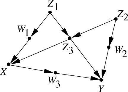
image 3

In SCM, if an undirected path connecting X and Y has an arrow pointing to X , then we call this path a backdoor path from X to Y. According to the normal causal chain, the structure of "X leads to Y" should be X→V1→V2→...→Vk−1→Vk→Y; however, if there is a backdoor path between X and Y, then the actual result is very False statistical correlations may arise.

Therefore, when a variable set S meets the following two conditions, we say that S meets the backdoor criterion:

S does not include descendants of X.

S can d separate all backdoor paths from X to Y.

For example, in Figure 3, sets such as {Z1,Z2,Z3},{Z1,Z3},{W1,Z3},{W2,Z3} all satisfy the backdoor criterion, but {Z3} does not.

The importance of the backdoor criterion is that it further generalizes the formula at the end of 2.5.3. If S satisfies the backdoor criterion from X to Y, then we can derive:

P(Y=y|do(X=x),S=s)=P(Y=y|X=x,S=s)

P(Y=y|do(X=x))=∑sP(Y=y|X=x,S=s)P(S=s)=∑sP(Y=y,X=x,S=s)P(X=x,S=s)

This greatly simplifies the calculation of SCM derivation.

2.6. Counterfactual Reasoning in SCM

The core of counterfactual inference is: Although X=x1 in reality, what happens to Y if X=x2?

Some people regret, "If I... then, I can..." This way of thinking is counterfactual reasoning.

Counterfactual inference is closely related to FPCI (the fundamental problem of causal inference). For a sample u that has received the intervention of the experimental group, we can only observe u's Yt(u), but never Yc(u), and vice versa. RCM (Virtual Fact Model) has a certain description of counterfactual reasoning, but RCM as a whole is not as clear, clear, and easy to explain as SCM.

Below, I will reformulate the interventionist causal view mentioned in Section 2.2 in terms of SCM .

The objects considered by RCM are all individuals u in a population U. In many cases, the assumption of homogeneity does not hold and each individual is different. In SCM, individual differences will be represented by the error term UV (the exogenous variable UV will correspondingly affect the endogenous variable V). Apart from the UVs, the "laws of nature" represented by the model M itself remain unchanged.

The RCM expression Yt(u) can be expressed as M.query(P(Y|do(T=t),U=u)) . That is: we intervene in the model M so that the variable T is assigned the value t; at the same time, we observe that the value of all exogenous variables U is u; in this case, we query the conditional probability of the variable Y we are interested in to the model M.

RCM requires models to have a default state of "no intervention". Obviously, SCM meets the requirements: Yc(u)=M.query(P(Y|U=u))

Therefore, SCM can answer counterfactual questions like "What is the value of Y if X = x1 instead of X = x0 in reality?" However, in real life, since the individual information U=u is usually unknown, and complex nonlinear structural equations may change with the distribution of U, counterfactual reasoning is generally difficult.

In conclusion, all RCMs can be expressed in SCM, and the white box of SCM is clearer and more stable than the black box of RCM.

3. Process causality

In Chapter 2, we used the SCM (Structural Causal Model) based on three basic intuitions:

Both cause and effect are separate events at separate points in time

The cause comes first, the result comes later

(obtained from 1 and 2) Two events cannot be mutually causal

However, in other situations, such as the number of predators and the number of prey, the two variables seem to "reciprocally cause and effect". SCM and Bayesian networks do not allow the existence of loops, so they cannot express such intuitive causal relationships. Therefore, we need a more complex causal model - Causal Loop Diagram (CLD for short) .

The variables in CLD are based on the following intuition:

cause and effect are certain processes that have a duration

Duration periods of cause and effect can overlap each other

Two processes can be mutually causal, and even a process itself can form a causal loop

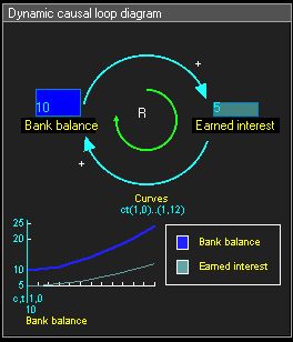
Causal Loop Diagram: Bank Deposits and Interest

Compared with SCM, CLD has not yet had such a rigorous and extensive theoretical framework. We can understand CLD as a function mapping "from a time scalar (real number) to an SCM set". For the convenience of modeling, all variables are numerical variables, and the interaction between multiple process variables is often linear, such as Y=αX+β. If α=dYdX>0, then we say that the link from X to Y is a positive link ; if α=dYdX<0, then we say that the link from X to Y is a negative link .

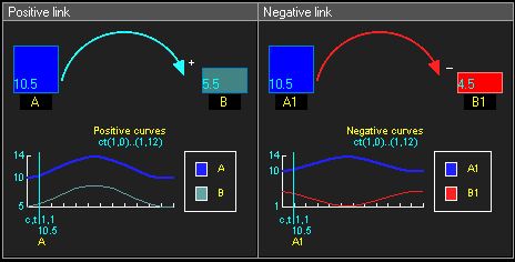
Positive links (left) and negative links (right)

For a causal loop A→B→A:

If an initial small increase (or decrease) in A leads through a causal loop leading to a further increase (or decrease) in A, then we call it a reinforcing feedback loop .
If an initial increase (or decrease) in A goes through a causal loop and instead causes A to decrease (or increase), thereby neutralizing the initial increase (or decrease), then we call it a balancing feedback loop .

Assuming A>0 and B>0, then:

If the A→B and B→A links are both positive and negative , then we can usually get a reinforcing feedback loop.
If the A→B and B→A links are positive and negative , then we can usually get a balanced feedback loop.

More generally, in a causal loop graph:

If there is an even number of negative links , then it is a reinforcing feedback loop.
If there is an odd number of negative links , then it's a balancing feedback loop.

The practical meaning of a feedback loop is usually as follows:

Reinforced feedback loops usually mean exponential growth, exponential decay , such as "revolving" bank deposits and interest, unrestricted population growth.
Balancing a feedback loop usually means reaching some equilibrium state , such as the solution of the Lotka-Volterra equation.

In the future, a possible research direction is to extend the more mature and extensive causal inference framework in SCM to CLD. The research focuses on introducing nonlinear, non-parametric complex causal links. Such research is necessarily difficult, but as computing power increases, we will gradually be able to construct more complex CLDs.

Reference materials, further reading:

https://yinguo.grandhoo.com/home

CS228 Notes

An Introduction to Causal Inference

Probabilistic Graphical Models: Principles and Techniques

Causality - Judea Pearl

The Art and Science of Cause and Effect - Judea Pearl

postscript

After reading this literature, I realized that many seemingly difficult philosophical questions may have good enough answers in other fields (economics, artificial intelligence, sociology, statistics, psychology, epidemiology, etc.) . Therefore, no matter what subject we are studying, we cannot be limited by the one-acre three-point land under our feet. On the contrary, we should draw more inspiration from different disciplines , and refrain from labeling ourselves as "only studying xxxx fields" and being complacent.

At the same time, we should also realize that when studying abstract and advanced subjects such as metaphysics, it is easy to have a false sense of superiority , thinking that we are superior to those who "only know the practical application", thus ignoring the importance of practice. importance. This approach is not advisable-for example, I cannot ignore data mining tuning skills because of the study of causality... In short, look up at the stars and keep your feet on the ground .

If you like it, you may wish to like it so that more people can see it; welcome to follow me.