
In the last blog, the author introduced the standard particle swarm and its implementation, and gave many improvement directions. From this issue, the improvement on particle swarm will be updated successively. There are three main directions for improvement in this issue. 1 . Chaotic initialization Particle swarm
2 Non-linear adjustment of inertial weight
3 Dynamic change of learning factor.
These improvement strategies are described in detail below.
00 Article Directory
1 Particle swarm improvement strategy
2 Code directory
3 Problem import
4 Simulation
5 Source code acquisition
01 Particle swarm improvement strategy
Particle swarm optimization algorithm shows great advantages in solving complex optimization problems. But like other intelligent algorithms, particle swarm optimization algorithm also has defects that are difficult to overcome, such as premature problems.
The values of parameters such as inertia weight and learning factor in the PSO algorithm play a very important role in the convergence performance of the algorithm, and researchers mostly use conventional values for these parameters, which will inevitably affect the convergence and convergence speed of the algorithm. Initialization also has a great impact on its accuracy and speed, and the uneven distribution of the solution space tends to fall into local optimum.
1.1 Chaos initialization
The traditional particle swarm optimization algorithm generally uses random initialization to determine the position distribution of the initial population, and the random number is generated by the computer, and then the initial position of each particle is randomly generated according to the following formula.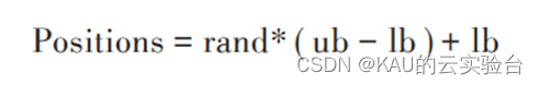
Positions represents the generated particle position; rand represents the generated random number, the value range is [0, 1]; ub, lb are the upper and lower bounds of the solution space, respectively.
Usually this kind of random initialization can generate a different initial population each time, which is more convenient to use. But there are also disadvantages, that is, the distribution of initial particles in the solution space is not uniform, and it is often encountered that the particles in a local area are too dense, and at the same time, the initial particles in a part of the area are too sparse. Such a situation is very unfavorable to the early convergence of the optimization algorithm. For the group optimization algorithm that is easy to fall into local optimum, it may lead to a decrease in the convergence speed or even failure to converge.
Chaotic initialization can effectively avoid these problems. Chaotic initialization has the characteristics of randomness, ergodicity and regularity. It traverses the search space within a certain range according to its own rules without repetition. The initial population generated in this way has obvious improvements in solution accuracy and convergence speed. The chaos initialization in this paper uses the Logistic chaos model, and its formula is as follows:
Among them, lamda is the mapping parameter of chaotic model. If μ∈[3.57,4], the system is in chaotic state; if μ=4, the system is in complete chaotic state. Generally take μ as 4.
The solution space distribution diagram generated by the above two initialization methods is as follows: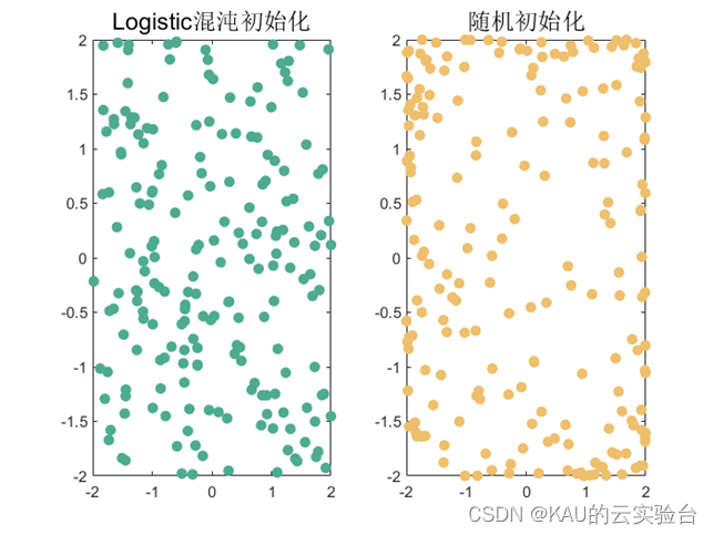
It can be seen that the distribution of the solution space after chaotic initialization is more uniform than that of random initialization, and there is no too dense or too sparse area.
1.2 Adaptive inertia weight
The inertia weight factor affects the performance of the PSO algorithm. A larger value is beneficial to the global search, and a smaller weight value is conducive to accelerating the convergence speed of the algorithm, which is more beneficial to the local meticulous development.
In order to balance the global search ability and local improvement ability of the PSO algorithm, a nonlinear dynamic inertia weight coefficient formula is used, and its expression is: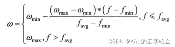
Among them, f represents the real-time objective function value of the particle, and favg and fmin represent the average value and minimum target value of all current particles, respectively. It can be seen from the above formula that the inertia weight changes with the change of particle objective function value. When the particle target value is scattered, reduce the inertia weight; when the particle target value is consistent, increase the inertia weight.
1.3 Dynamic Learning Factor
In the standard particle swarm optimization algorithm, c1 and c2 are learning factors, which generally take fixed values. The learning factor c1 represents the particle’s thinking about itself, that is, the part that the particle learns from itself; the learning factor c2 reflects the social nature of the particle, that is, the particle Features learned from the globally optimal particle.
During the process of the particle swarm optimization algorithm, the algorithm should search extensively in space at the beginning to increase the diversity of particles, and in the later stage, it should pay attention to the convergence of the algorithm, which is reflected in the algorithm. The learning factors c1 and c2 should be weighted as the algorithm progresses Values are variable and should not be fixed.
Therefore, in order to prevent the particles from quickly gathering around the local optimal solution in the early stage of evolution and make the particles search in a large range in the global field, let c1 take a larger value and c2 take a smaller value. In the later stage of the search, in order to make the particles converge to the global optimal solution quickly and accurately, and improve the convergence speed and accuracy of the algorithm, set c1 to a smaller value and c2 to a larger value. Therefore, in this paper, C1 is constructed as a monotonically decreasing function, and C2 is constructed as a monotonically increasing function. The expressions of the two are as follows: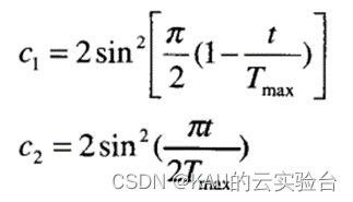
where t is the current iteration number. Tmax is the maximum number of iterations of the particle swarm. It can be seen from the above that by dynamically adjusting the value of the learning factor, the group can quickly search for the optimal value in a short period of time in the early stage of evolution, and quickly and accurately converge to the optimal solution in the later stage of evolution.
C1, C2 function images are as follows: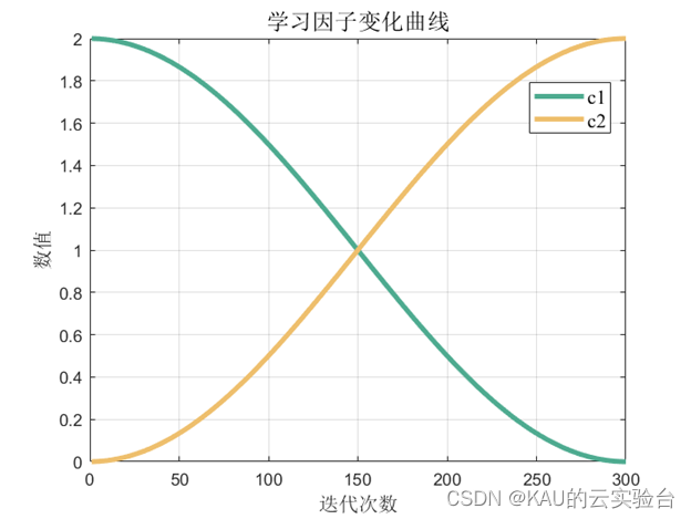
02 Code Directory
First run main_ipso.m and main_pso.m, and then run compare.m to see the iterative comparison
03 Question import
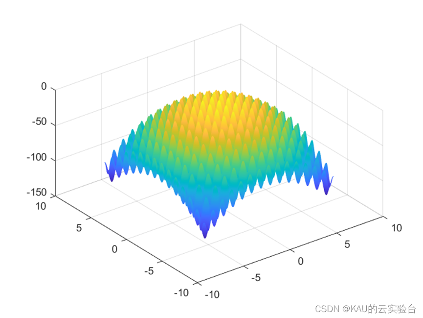
In order to verify the performance of the algorithm, a commonly used test function Rastrigrin function in Benchmark is used: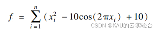

'
If the function is negative, the greater the fitness, the better.
This function is a multimodal function and converges to (0,0,...,0).
04 Simulation
Add the above improved strategy to the standard particle swarm, and compare it through the Rastrigrin function, and get the following results: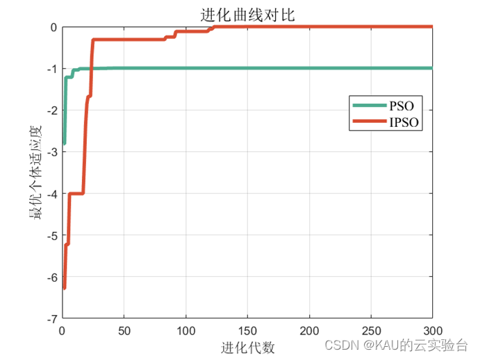
Among them, the value and fitness of IPSO are: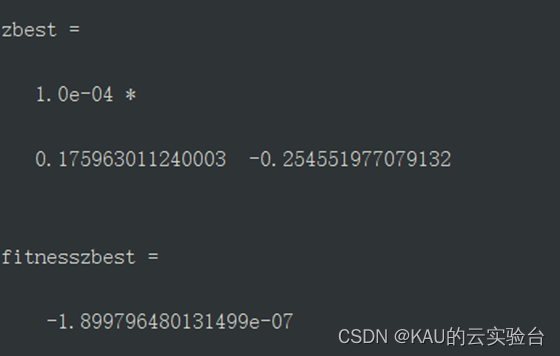
The value and fitness of PSO are: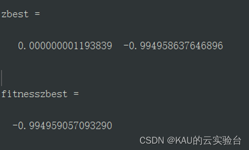
Obviously, PSO is trapped in local optimum, and it is difficult to escape from the local solution. Adaptive chaotic particle swarm algorithm has better performance.
05 Source code acquisition
%%%%%%%%%%%%%%%%%%%%%%%%%%%%%%%%%%%%%%%%%%%%%%%%%%%%%%%%%%%%%%%%%%
https://mbd.pub/o/bread/ZJqbmpdv
%%%%%%%%%%%%%%%%%%%%%%%%%%%%%%%%%%%%%%%%%%%%%%%%%%%%%%%%%%%%%%%%%%
If this article is helpful or inspiring to you, you can click the Like (ง •̀_•́)ง (you don’t need to click) in the lower right corner. If you have customization needs, you can private message the author.