Vgg16 recognizes 4 simple eye expressions (TensorFlow)

Project data and source code

Available for download on github:

https://github.com/chenshunpeng/Recognition-of-eye-state-based-on-Vgg16

1. Data processing

1.1. Data introduction

There are a total of 4 kinds of eye expressions, which are closed eyes, forward, left, and right. The data are introduced as follows:

Eye_dataset
    ├── close_look
    │   └── eye_closed (XXX).XXX（1,148 张图片，共4.15 MB）
    │ 
    ├── forward_look
    │   └── forward_look (XXX).XXX（1,038 张图片，共7.37 MB）
    │ 
    ├── left_look
    │   └── left_(XXX).XXX（1,049 张图片，共11.0 MB）
    │         
    ├── right_look
    └── └──	right_(XXX).XXX（1,073 张图片，共9.69 MB）

1.2. Import data

Check tensorflow version:

import tensorflow as tf
tf.__version__

Version:'2.9.1'

Let’s popularize the advantages and disadvantages of Keras and PyTorch: (For details, see: Portal )

In some cases, you need to find a specific model in a specific machine learning domain.

For example, when doing an object detection competition and wanted to implement DETR (Facebook's Data-Efficient transformer), it turned out that most of the resources were written in PyTorch, so in this case, it was easier to use PyTorch.

Also, PyTorch's code implementations are longer because they cover many low-level details, which is both an advantage and a disadvantage. When you're a beginner, it's very helpful to learn the low-level details before moving on to higher-level APIs such as Keras.

However, this is also a disadvantage, as you can find yourself lost in many details and rather long code segments. So essentially, if you're working on a tight deadline, it's better to choose Keras over PyTorch.

Set up the GPU environment:

import tensorflow as tf

gpus = tf.config.list_physical_devices("GPU")
if gpus:
    tf.config.experimental.set_memory_growth(gpus[0], True)  #设置GPU显存用量按需使用
    tf.config.set_visible_devices([gpus[0]],"GPU")

# 打印显卡信息，确认GPU可用
print(gpus)

output:[PhysicalDevice(name='/physical_device:GPU:0', device_type='GPU')]

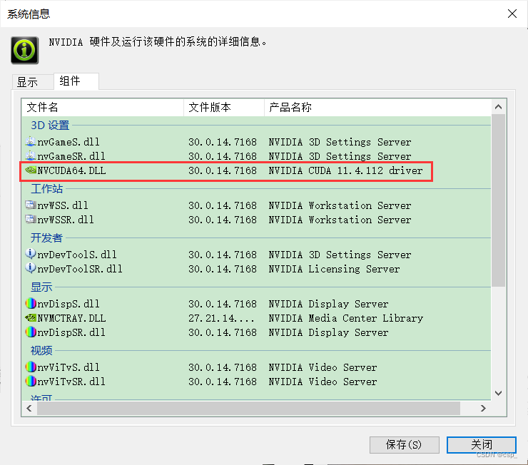
Briefly introduce the environment I configured:

The cuda supported by my computer (open nvidia (right click on the desktop) -> select system information in the lower left corner -> components)

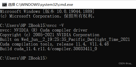
nvcc -VCheck the downloaded CUDA version:

Then install cuDNN, register and download from the official website:

first cd C:\Program Files\NVIDIA GPU Computing Toolkit\CUDA\v11.4\extras\demo_suite, after executingbandwidthTest.exe

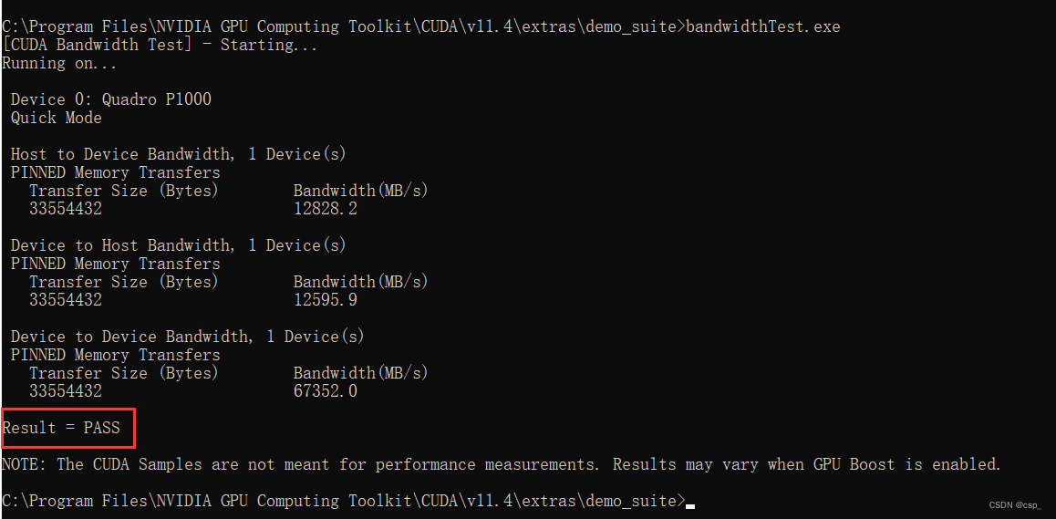
implementdeviceQuery.exe

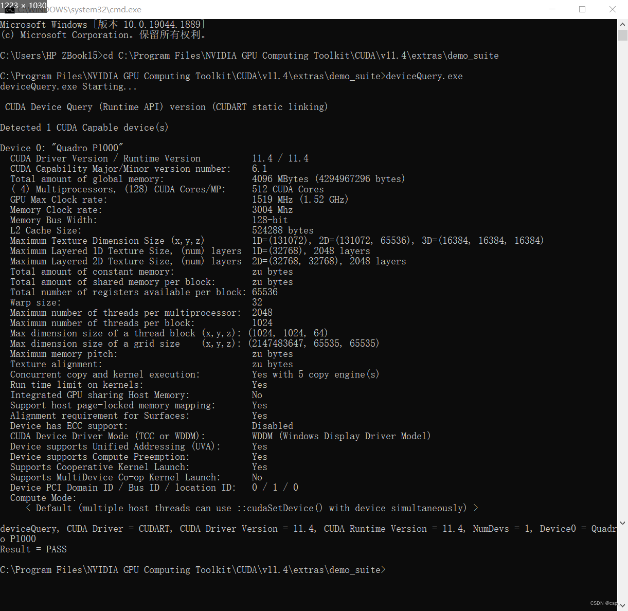
If the 2 PASS above appear, it means that cuDNN is successfully installed

Import and view data:

For the use of random number seeds, see: Tensorflow application – usage of tf.set_random_seed

import matplotlib.pyplot as plt
# 支持中文
plt.rcParams['font.sans-serif'] = ['SimHei']  # 用来正常显示中文标签
plt.rcParams['axes.unicode_minus'] = False  # 用来正常显示负号

import os,PIL

# 设置随机种子尽可能使结果可以重现
import numpy as np
np.random.seed(1)

# 设置随机种子尽可能使结果可以重现
import tensorflow as tf
# tf.random.set_seed:设置全局随机种子
tf.random.set_seed(1)

import pathlib

data_dir = "E:\demo_study\jupyter\Jupyter_notebook\Recognition-of-eye-state-based-on-CNN\Eye_dataset"
data_dir = pathlib.Path(data_dir)

# */*的意思为获取文件夹下的所有文件及它们的子文件
# https://blog.csdn.net/Crystal_remember/article/details/116804009
image_count = len(list(data_dir.glob('*/*')))
print("图片总数为：",image_count)

output:图片总数为： 4308

1.3. Data preprocessing

Initialization parameters:

batch_size = 8
img_height = 224
img_width = 224

image_dataset_from_directoryLoad data from disk tf.data.Datasetinto the

Function prototype:

tf.keras.preprocessing.image_dataset_from_directory(
    directory,
    labels="inferred",
    label_mode="int",
    class_names=None,
    color_mode="rgb",
    batch_size=32,
    image_size=(256, 256),
    shuffle=True,
    seed=None,
    validation_split=None,
    subset=None,
    interpolation="bilinear",
    follow_links=False,
)

Official website introduction: tf.keras.utils.image_dataset_from_directory

For validation_splititems, the official website explains: Optional float between 0 and 1, fraction of data to reserve for validation.

For subsetitems, the official website explains: Subset of the data to return. One of “training” or “validation”. Only used if validation_splitis set.

This part of code:

train_ds = tf.keras.preprocessing.image_dataset_from_directory(
    data_dir, #WindowsPath('E:/demo_study/jupyter/Jupyter_notebook/Recognition-of-eye-state-based-on-CNN/Eye_dataset')
    validation_split=0.2,
    subset="training",
    seed=12,
    image_size=(img_height, img_width),
    batch_size=batch_size)

output:

Found 4308 files belonging to 4 classes.
Using 3447 files for training.

Configure the verification set in the same way:

val_ds = tf.keras.preprocessing.image_dataset_from_directory(
    data_dir,
    validation_split=0.2,
    subset="validation",
    seed=12,
    image_size=(img_height, img_width),
    batch_size=batch_size)

output:

Found 4308 files belonging to 4 classes.
Using 861 files for validation.

We can pass class_namesthe labels of the output dataset, the labels will correspond to the directory names in alphabetical order

class_names = train_ds.class_names
print(class_names)
class_names = val_ds.class_names
print(class_names)

output:

['close_look', 'forward_look', 'left_look', 'right_look']
['close_look', 'forward_look', 'left_look', 'right_look']

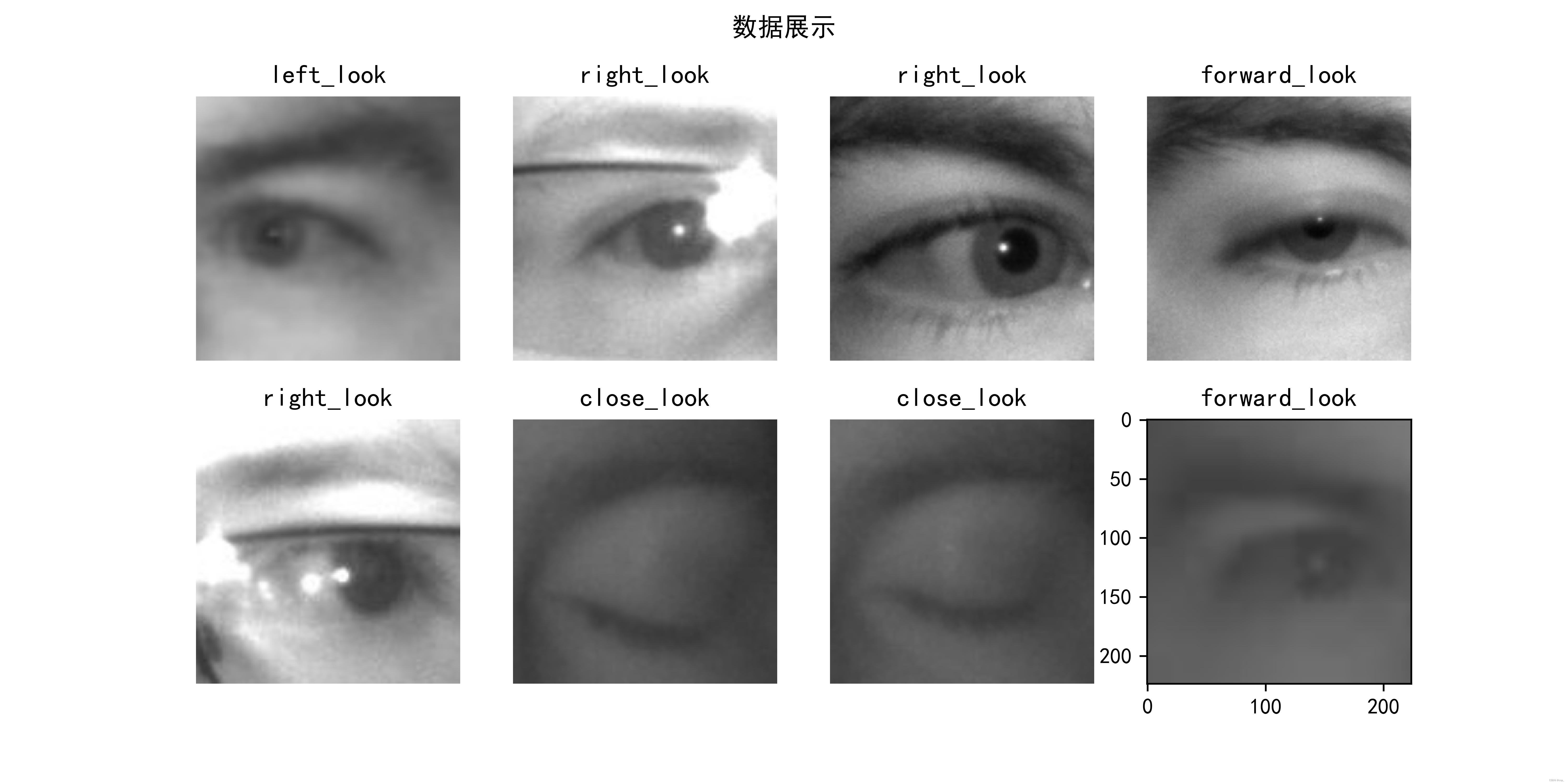
1.4. Visualizing data

plt.figure(figsize=(10, 5))  # 图形的宽为10高为5
plt.suptitle("数据展示")

for images, labels in train_ds.take(1):
    for i in range(8):
        ax = plt.subplot(2, 4, i + 1)  
        plt.imshow(images[i].numpy().astype("uint8"))
        plt.title(class_names[labels[i]])
        plt.savefig('pic1.jpg', dpi=600) #指定分辨率保存
        plt.axis("off")

result:

View the respective data formats for images and labels:

for image_batch, labels_batch in train_ds:
    print(image_batch.shape)
    print(labels_batch.shape)
    break

output:

(8, 224, 224, 3)
(8,)

explain:

• Image_batchIs a tensor of shape (8, 224, 224, 3), that is, a batch of 8 images with a shape of 240x240x3 (the last dimension refers to the color channel RGB)
• Label_batchIs a tensor of shape (8,), that is, the label corresponding to 8 pictures

1.5. Configure Dataset

shuffle(): Shuffle the data, for details, please refer to: The understanding of buffer_size in the data set shuffle method

prefetch(): Prefetch data to speed up operation. For details, please refer to: Better performance with the tf.data API

cache(): Cache the data set into the memory to speed up the operation

Recommend a blog: [Study Notes] Use tf.data to optimize the preprocessing process

prefetch()Detailed introduction of the function: it makes the preprocessing and model execution of the training step overlap, and it turns out to be:

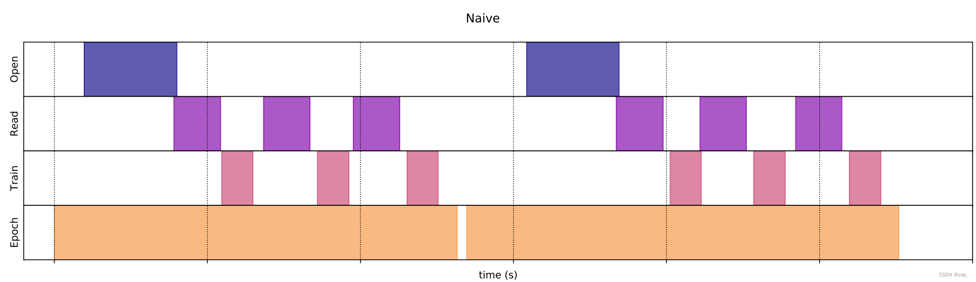
prefetch()followed by:

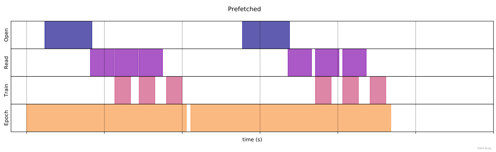
Of course, you can do otherwise

AUTOTUNE = tf.data.AUTOTUNE

train_ds = train_ds.cache().shuffle(1000).prefetch(buffer_size=AUTOTUNE)
val_ds   = val_ds.cache().prefetch(buffer_size=AUTOTUNE)

2. Network design

2.1.vgg16 brief introduction

See the paper for details: Very Deep Convolutional Networks for Large-Scale Image Recognition

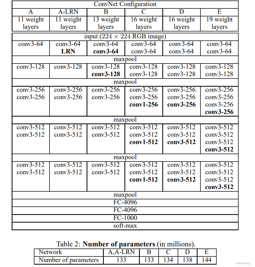
The VGG-16 architecture is as follows:

Specific process: (Borrowed from: Deep Learning - Detailed Explanation of VGG16 Model )

1. The input image size is 224x224x3, after 64 channels of 3x3 convolution kernels, the step size is 1, padding=same padding, convolution twice, and then activated by ReLU, the output size is 224x224x64
2. After max pooling (maximized pooling), the filter is 2x2, the step size is 2, the image size is halved, and the pooled size becomes 112x112x64
3. After 128 3x3 convolution kernels, two convolutions, ReLU activation, the size becomes 112x112x128
4. Max pooling pooling, the size becomes 56x56x128
5. After 256 3x3 convolution kernels, triple convolution, ReLU activation, the size becomes 56x56x256
6. Max pooling pooling, the size becomes 28x28x256
7. After 512 3x3 convolution kernels, triple convolution, ReLU activation, the size becomes 28x28x512
8. Max pooling pooling, the size becomes 14x14x512
9. After 512 3x3 convolution kernels, triple convolution, ReLU, the size becomes 14x14x512
10. Max pooling pooling, the size becomes 7x7x512
11. Then Flatten(), flatten the data into a vector and become one-dimensional 51277=25088.
12. After two layers of 1x1x4096 and one layer of 1x1x1000 fully connected layers (a total of three layers), activated by ReLU
13. Finally, output 1000 prediction results through softmax

From the above process, it can be seen that the VGG network structure is quite simple. It is composed of small convolution kernels, small pool kernels, and ReLU. The simplified diagram is as follows (also the network structure used in this article):

2.2. Training

Call the official vgg16 network model

model = tf.keras.applications.VGG16()
# 打印模型信息
model.summary()

That is, the D model in the figure below:

output:

Model: "vgg16"
_________________________________________________________________
 Layer (type)                Output Shape              Param #   
=================================================================
 input_1 (InputLayer)        [(None, 224, 224, 3)]     0         
                                                                 
 block1_conv1 (Conv2D)       (None, 224, 224, 64)      1792      
                                                                 
 block1_conv2 (Conv2D)       (None, 224, 224, 64)      36928     
                                                                 
 block1_pool (MaxPooling2D)  (None, 112, 112, 64)      0         
                                                                 
 block2_conv1 (Conv2D)       (None, 112, 112, 128)     73856     
                                                                 
 block2_conv2 (Conv2D)       (None, 112, 112, 128)     147584    
                                                                 
 block2_pool (MaxPooling2D)  (None, 56, 56, 128)       0         
                                                                 
 block3_conv1 (Conv2D)       (None, 56, 56, 256)       295168    
                                                                 
 block3_conv2 (Conv2D)       (None, 56, 56, 256)       590080    
                                                                 
 block3_conv3 (Conv2D)       (None, 56, 56, 256)       590080    
                                                                 
 block3_pool (MaxPooling2D)  (None, 28, 28, 256)       0         
                                                                 
 block4_conv1 (Conv2D)       (None, 28, 28, 512)       1180160   
                                                                 
 block4_conv2 (Conv2D)       (None, 28, 28, 512)       2359808   
                                                                 
 block4_conv3 (Conv2D)       (None, 28, 28, 512)       2359808   
                                                                 
 block4_pool (MaxPooling2D)  (None, 14, 14, 512)       0         
                                                                 
 block5_conv1 (Conv2D)       (None, 14, 14, 512)       2359808   
                                                                 
 block5_conv2 (Conv2D)       (None, 14, 14, 512)       2359808   
                                                                 
 block5_conv3 (Conv2D)       (None, 14, 14, 512)       2359808   
                                                                 
 block5_pool (MaxPooling2D)  (None, 7, 7, 512)         0         
                                                                 
 flatten (Flatten)           (None, 25088)             0         
                                                                 
 fc1 (Dense)                 (None, 4096)              102764544 
                                                                 
 fc2 (Dense)                 (None, 4096)              16781312  
                                                                 
 predictions (Dense)         (None, 1000)              4097000   
                                                                 
=================================================================
Total params: 138,357,544
Trainable params: 138,357,544
Non-trainable params: 0
_________________________________________________________________

Set dynamic learning rate

# 设置初始学习率
initial_learning_rate = 1e-4

lr_schedule = tf.keras.optimizers.schedules.ExponentialDecay(
        initial_learning_rate, 
        decay_steps=20,      # 注意这里是指 steps，不是指 epochs
        decay_rate=0.96,     # lr经过一次衰减就会变成 decay_rate*lr
        staircase=True)

# 将指数衰减学习率送入优化器
optimizer = tf.keras.optimizers.Adam(learning_rate=lr_schedule)

model compilation

• Loss function (loss): It is used to measure the accuracy of the model during training. It is used here sparse_categorical_crossentropy. The principle categorical_crossentropyis the same as (multi-class cross-entropy loss), but the integer code used for the real value (for example, the 0th class is represented by the number 0, and the 0th class is represented by the number 0. The 3 classes are represented by the number 3, which can be seen officially: tf.keras.losses.SparseCategoricalCrossentropy）
• Optimizer (optimizer): decides how the model is updated based on the data it sees and its own loss function, here it is Adam(officially available: tf.keras.optimizers.Adam )
• Evaluation function (metrics): used to monitor the training and testing steps, this time accuracy, the ratio of correctly classified images (officially available: tf.keras.metrics.Accuracy )

model.compile(optimizer=optimizer,
              loss     ='sparse_categorical_crossentropy',
              metrics  =['accuracy'])

training model

epochs = 10
history = model.fit(
    train_ds,
    validation_data=val_ds,
    epochs=epochs
)

here $step$（$iteration$ ) is:$step=\lceil \frac{exampleNums\ast epoch}{batchsize}\rceil =\lceil \frac{3447\ast 1}{8}\rceil =431$

output:

Epoch 1/10
431/431 [==============================] - 266s 604ms/step - loss: 0.4236 - accuracy: 0.8567 - val_loss: 0.1470 - val_accuracy: 0.9501
Epoch 2/10
431/431 [==============================] - 254s 589ms/step - loss: 0.0895 - accuracy: 0.9698 - val_loss: 0.0959 - val_accuracy: 0.9721
Epoch 3/10
431/431 [==============================] - 254s 589ms/step - loss: 0.0406 - accuracy: 0.9881 - val_loss: 0.0923 - val_accuracy: 0.9733
Epoch 4/10
431/431 [==============================] - 253s 587ms/step - loss: 0.0215 - accuracy: 0.9942 - val_loss: 0.1004 - val_accuracy: 0.9733
Epoch 5/10
431/431 [==============================] - 253s 587ms/step - loss: 0.0161 - accuracy: 0.9951 - val_loss: 0.0996 - val_accuracy: 0.9791
Epoch 6/10
431/431 [==============================] - 253s 587ms/step - loss: 0.0133 - accuracy: 0.9962 - val_loss: 0.1016 - val_accuracy: 0.9779
Epoch 7/10
431/431 [==============================] - 253s 587ms/step - loss: 0.0116 - accuracy: 0.9965 - val_loss: 0.1027 - val_accuracy: 0.9779
Epoch 8/10
431/431 [==============================] - 253s 587ms/step - loss: 0.0109 - accuracy: 0.9971 - val_loss: 0.1033 - val_accuracy: 0.9779
Epoch 9/10
431/431 [==============================] - 253s 587ms/step - loss: 0.0106 - accuracy: 0.9971 - val_loss: 0.1036 - val_accuracy: 0.9779
Epoch 10/10
431/431 [==============================] - 253s 587ms/step - loss: 0.0104 - accuracy: 0.9971 - val_loss: 0.1036 - val_accuracy: 0.9779

3. Model evaluation

3.1. Accuracy Evaluation

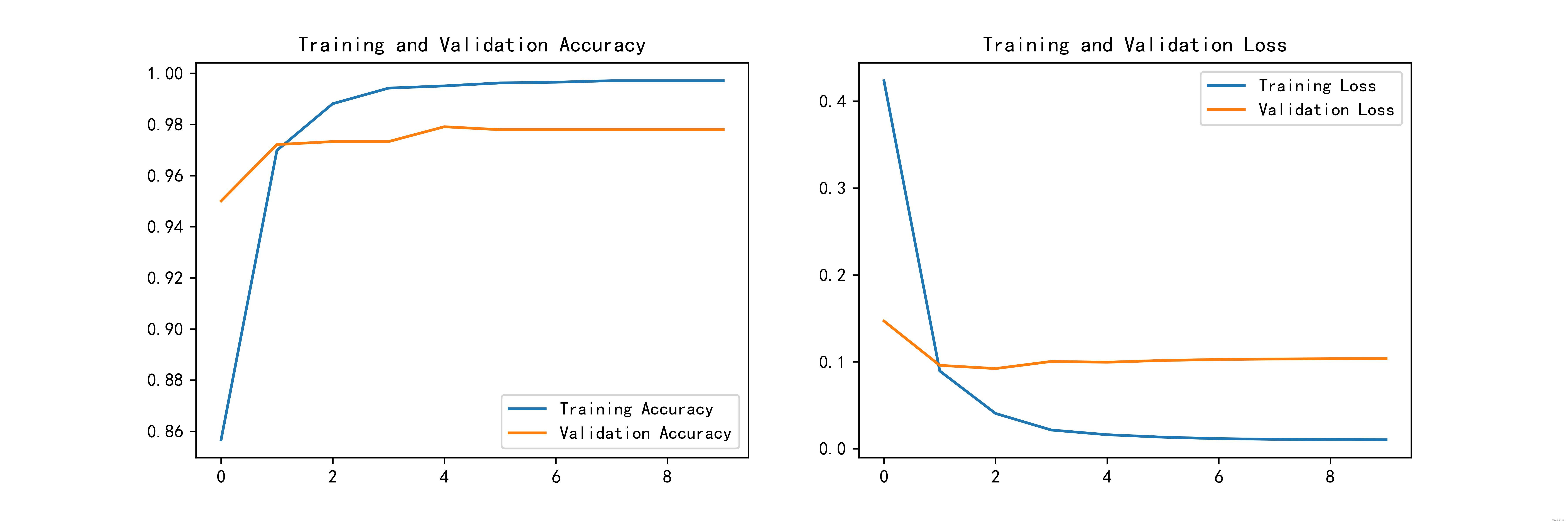
Accuracy and Loss graph

acc = history.history['accuracy']
val_acc = history.history['val_accuracy']

loss = history.history['loss']
val_loss = history.history['val_loss']

epochs_range = range(epochs)

plt.figure(figsize=(12, 4))
plt.subplot(1, 2, 1)

plt.plot(epochs_range, acc, label='Training Accuracy')
plt.plot(epochs_range, val_acc, label='Validation Accuracy')
plt.legend(loc='lower right')
plt.title('Training and Validation Accuracy')

plt.subplot(1, 2, 2)
plt.plot(epochs_range, loss, label='Training Loss')
plt.plot(epochs_range, val_loss, label='Validation Loss')
plt.legend(loc='upper right')
plt.title('Training and Validation Loss')
plt.savefig('pic2.jpg', dpi=600) #指定分辨率保存
plt.show()

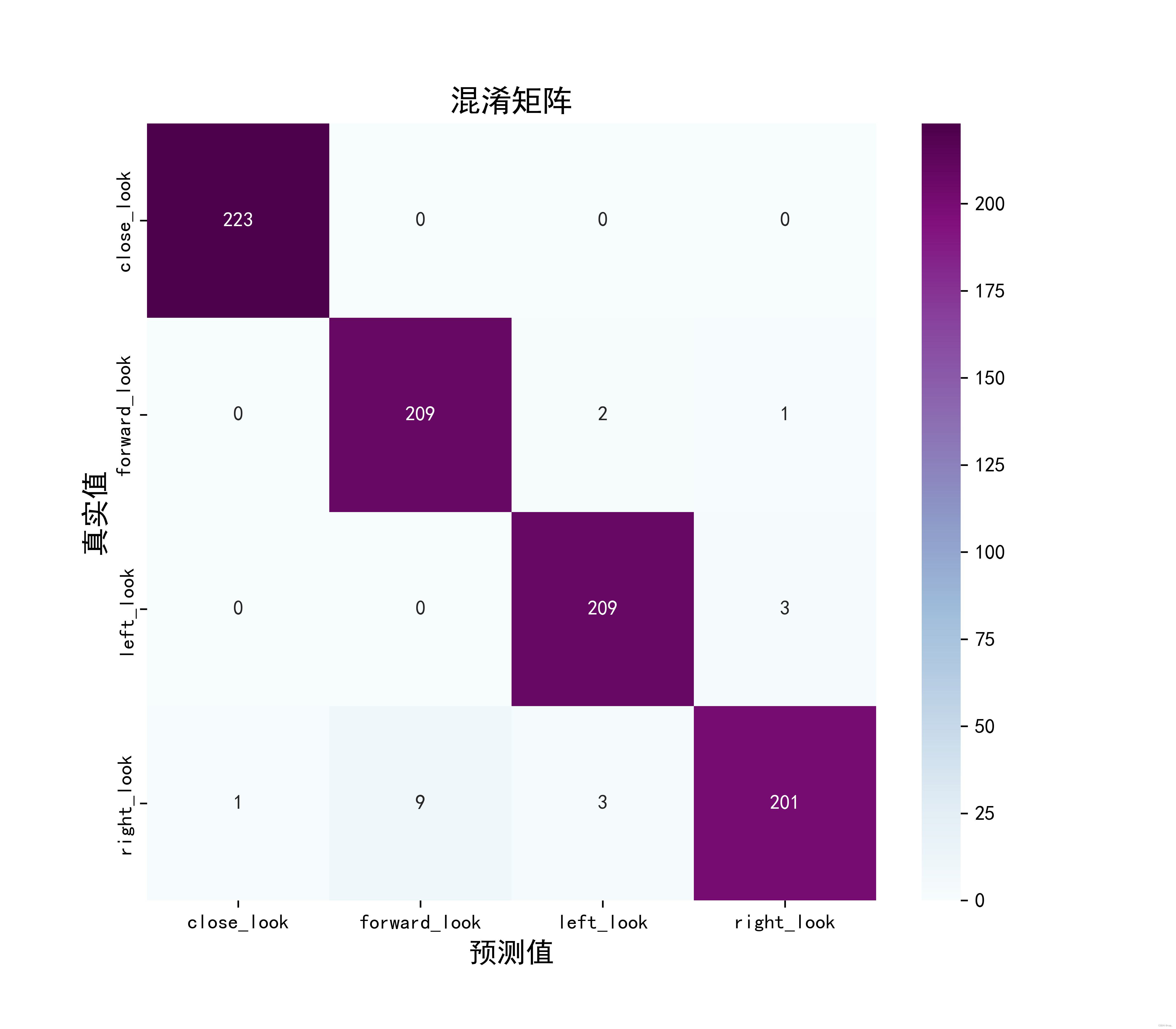
3.2. Draw the confusion matrix

confusion_matrix()The introduction can be seen: sklearn.metrics.confusion_matrix

Seaborn: Based on Matplotlibthe core library, a higher-level API package is carried out, and its advantages are more comfortable color matching and more delicate styles of graphic elements

Define a function to plot a confusion matrix plot_cm:

from sklearn.metrics import confusion_matrix
import seaborn as sns
import pandas as pd

def plot_cm(labels, predictions):
    
    # 生成混淆矩阵
    conf_numpy = confusion_matrix(labels, predictions)
    # 将矩阵转化为 DataFrame
    conf_df = pd.DataFrame(conf_numpy, index=class_names ,columns=class_names)  
    plt.figure(figsize=(8,7))
    sns.heatmap(conf_df, annot=True, fmt="d", cmap="BuPu")
    plt.title('混淆矩阵',fontsize=15)
    plt.ylabel('真实值',fontsize=14)
    plt.xlabel('预测值',fontsize=14)
    plt.savefig('pic3.jpg', dpi=600) #指定分辨率保存

Take part of the verification data ( .take(1)) to generate a confusion matrix:

val_pre   = []
val_label = []

for images, labels in val_ds:#这里可以取部分验证数据（.take(1)）生成混淆矩阵
    for image, label in zip(images, labels):
        # 需要给图片增加一个维度
        img_array = tf.expand_dims(image, 0) 
        # 使用模型预测图片中的人物
        prediction = model.predict(img_array)

        val_pre.append(class_names[np.argmax(prediction)])
        val_label.append(class_names[label])

Output (image processing):

1/1 [==============================] - 2s 2s/step
1/1 [==============================] - 0s 23ms/step
1/1 [==============================] - 0s 21ms/step
...

Take a look at conf_numpythe variables:

conf_numpy = confusion_matrix(val_label, val_pre)
conf_numpy

output:

array([[223,   0,   0,   0],
       [  0, 209,   2,   1],
       [  0,   0, 209,   3],
       [  1,   9,   3, 201]], dtype=int64)

Then call plot_cm()to draw:

plot_cm(val_label, val_pre)

Remember to save the model

# 保存模型
model.save('model/17_model.h5')

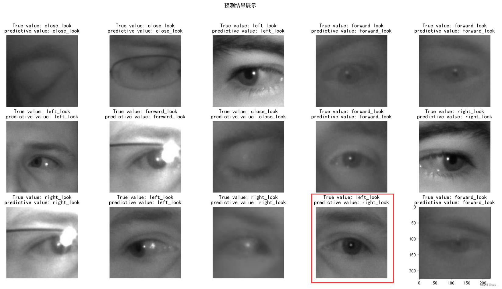
3.3. Making predictions

# model = tf.keras.models.load_model('model/17_model.h5')
plt.figure(figsize=(20, 10))  # 图形的宽为10高为5
plt.suptitle("预测结果展示")

num = -1
for images, labels in val_ds.take(2):
    for i in range(8):
        num = num + 1
        plt.subplots_adjust(left=None, bottom=None, right=None, top=None , wspace=0.2, hspace=0.2)
        if num >= 15:
            break
        ax = plt.subplot(3, 5, num + 1)  
        
        # 显示图片
        plt.imshow(images[i].numpy().astype("uint8"))
        
        # 需要给图片增加一个维度
        img_array = tf.expand_dims(images[i], 0) 
        
        # 使用模型预测图片中的人物
        predictions = model.predict(img_array)
        plt.title("True value: {}\npredictive value: {}".format(class_names[labels[i]],class_names[np.argmax(predictions)]))
        plt.savefig('pic4.jpg', dpi=600) #指定分辨率保存
        plt.axis("off")

Results (the red box is the case of prediction error):