Python traffic sign recognition system based on YOLOv5 [source code & technical documentation & deployment video & data set]

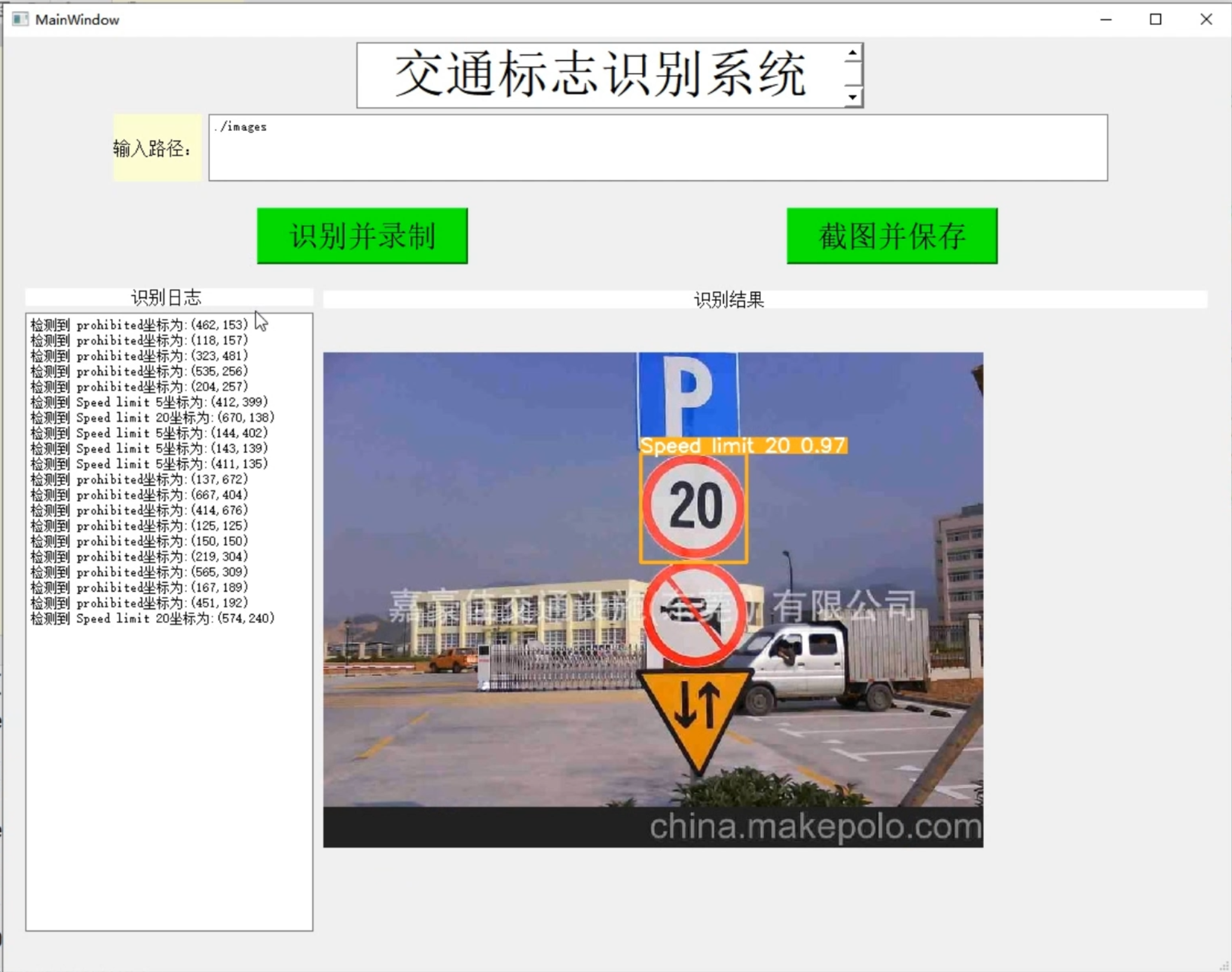
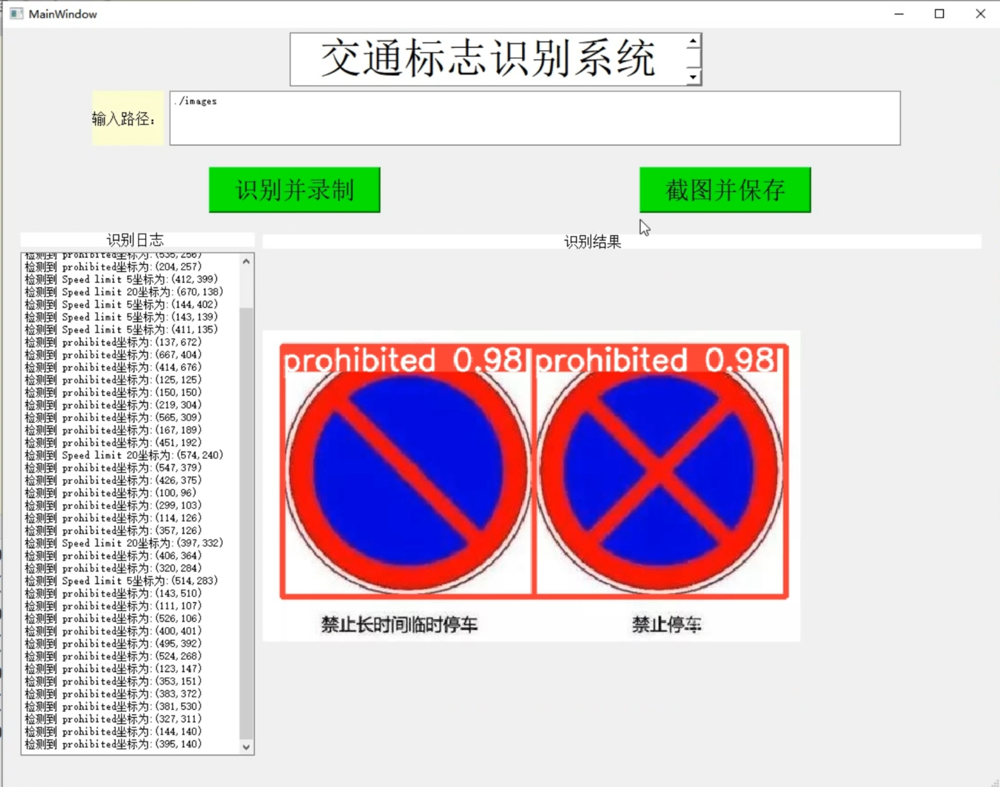
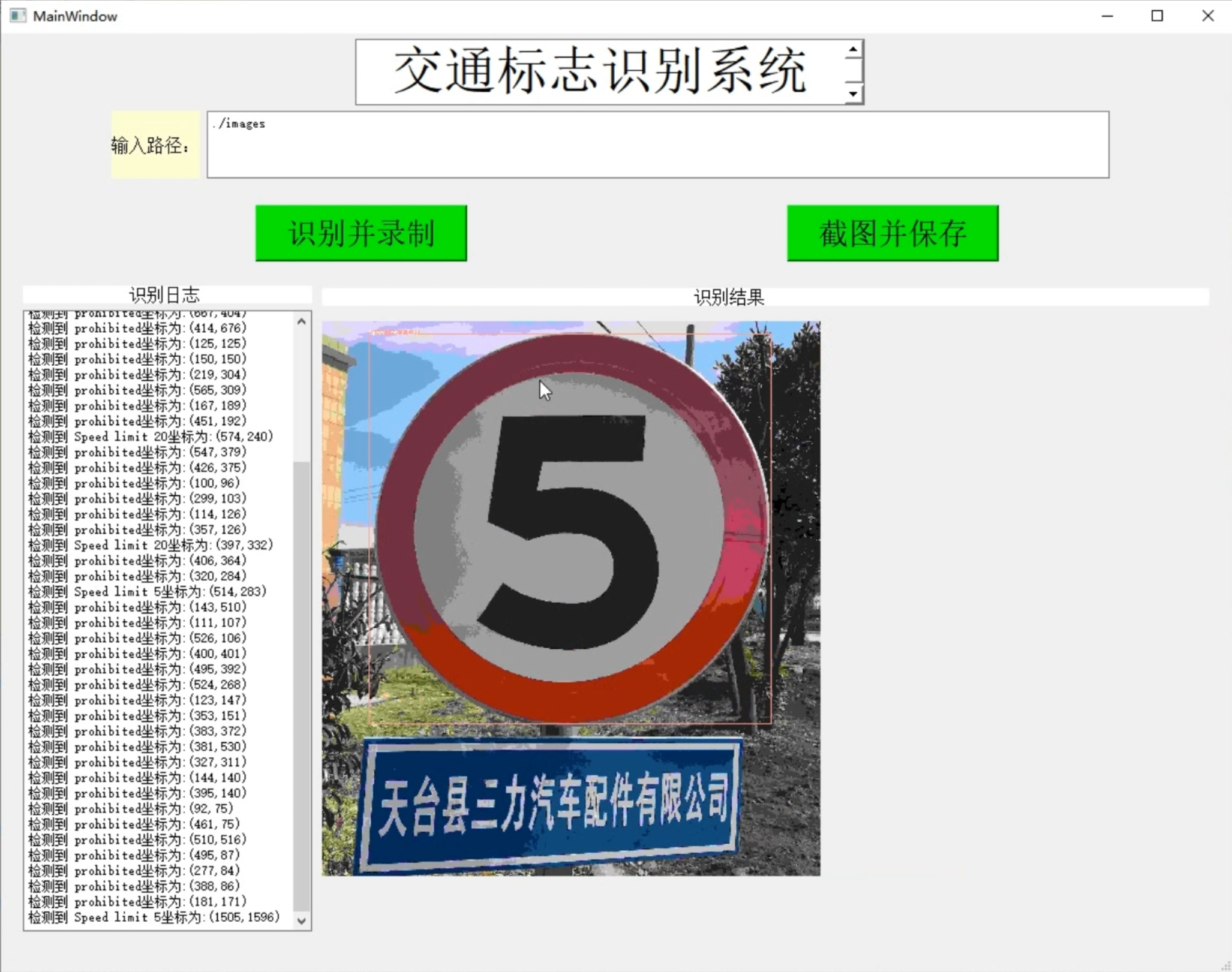
1. Picture demonstration:

2. Video demonstration:

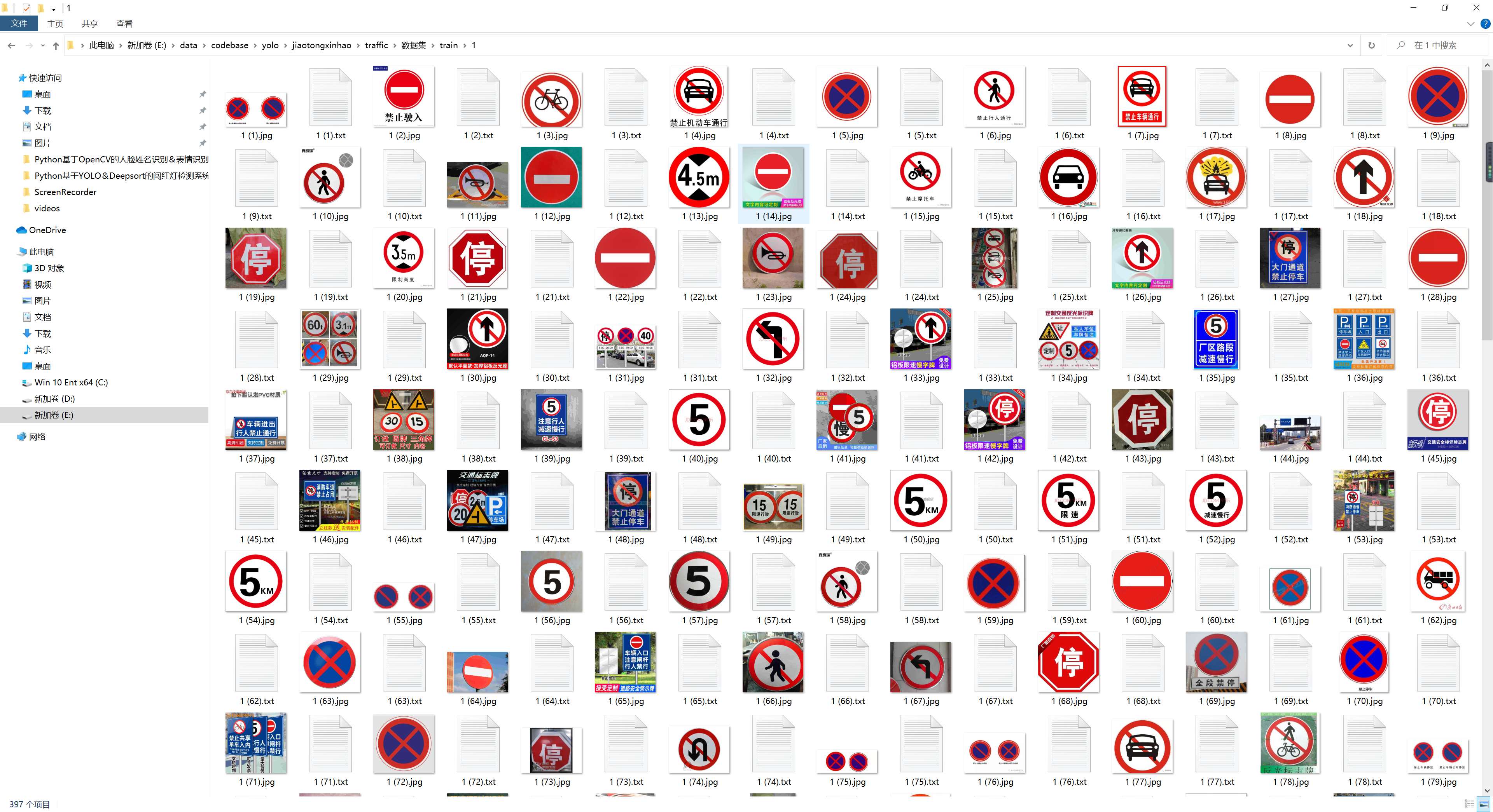
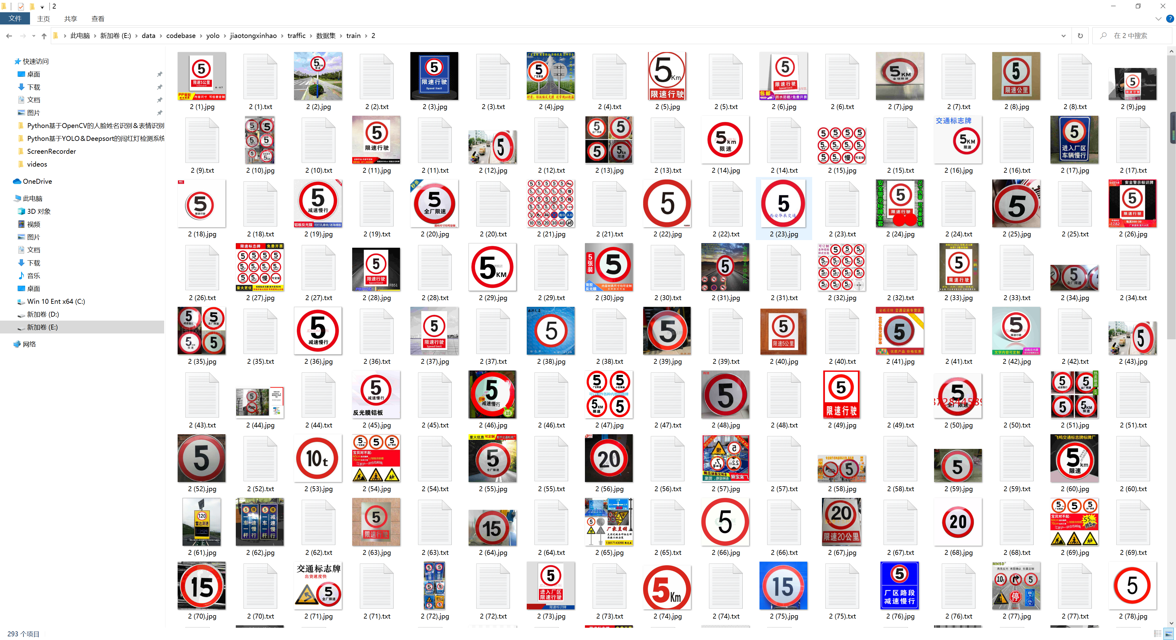
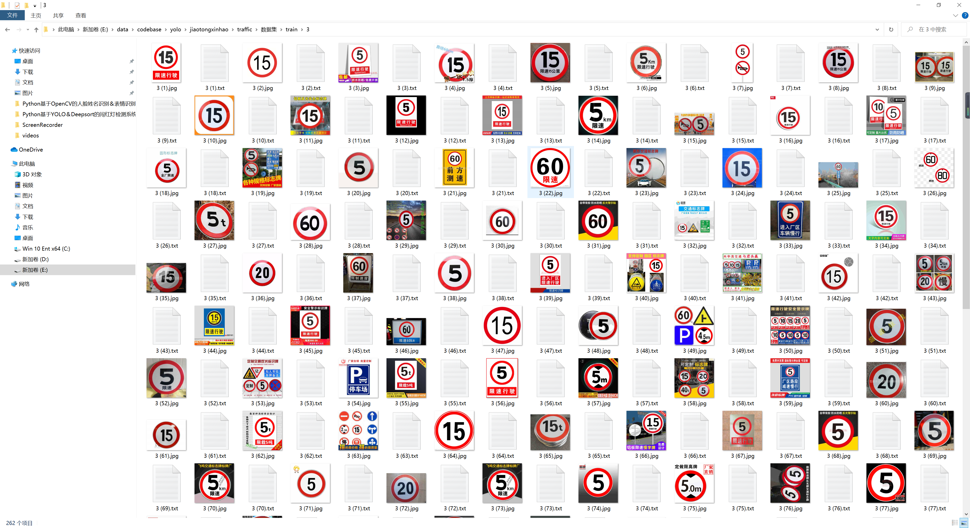
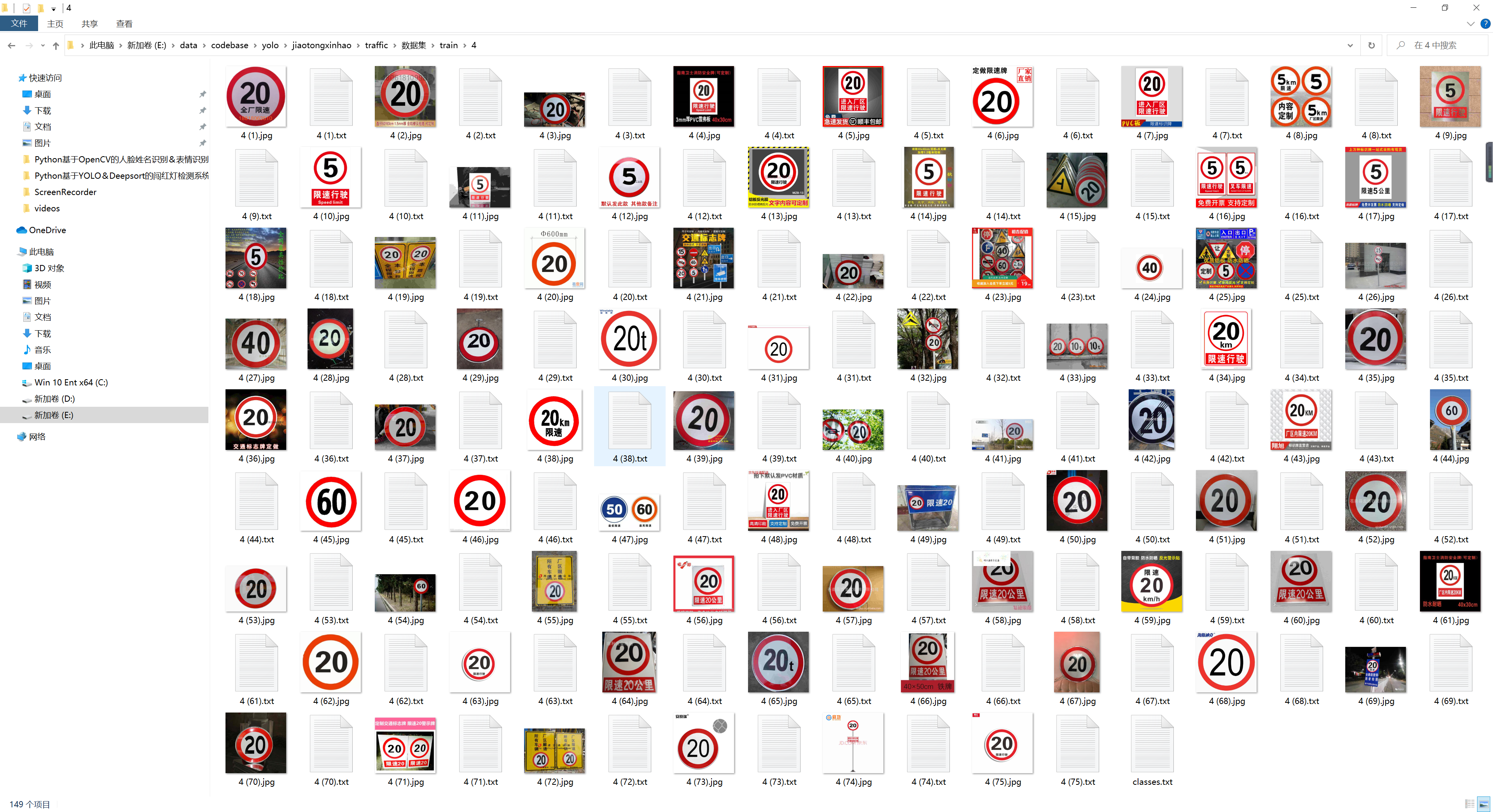
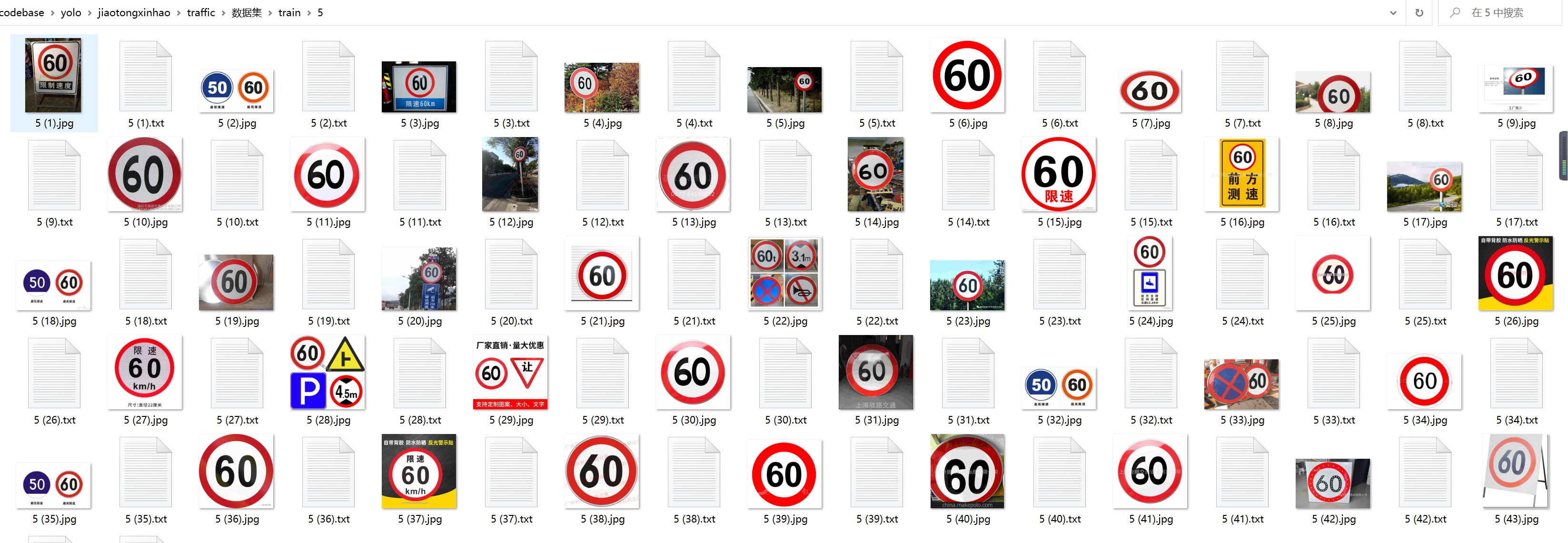
3. Labeled dataset:

4. Construction of YOLO network:

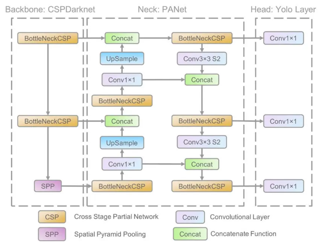
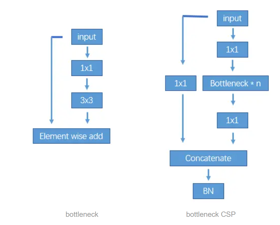
The network structure is to first use Focus to change the length and width of the calculation graph to 1/4 of the original, and multiply the number of channels by 4. Then use bottleneckCSP to extract features. Personally, I understand that CSP is the fusion of more different channels.

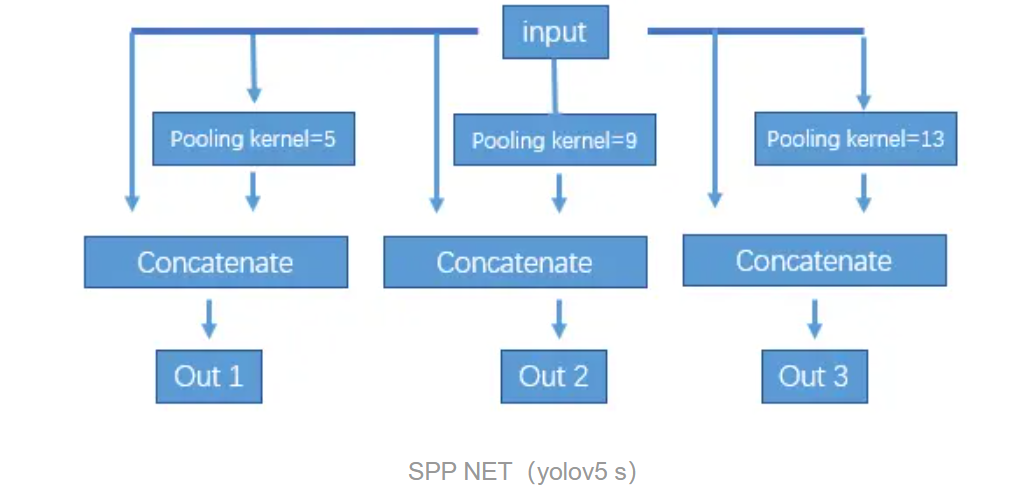
Then use maxpooling downsampling to build a feature pyramid. Downsampling over each stage with input cancatenate.

Then upsample the feature map generated by downsampling, and fuse it with the corresponding layer in the backbone. Finally, use the detect layer to predict anchors. The output channel of the detect layer is (class num + 5) * the number of anchors predicted by each grid per layer. num class is the probability that the predicted result is each class, and 5 is the confidence of the anchor's x, y, w, h and whether it is an object. The default configuration generates feature maps of three sizes after maxpooling. Each feature map is used to predict anchors after upsampling and fusion operations, and each grid predicts three anchors. For example, yolov5 s predicts that there are 80 types of anchors. Output x.shape=(bs, 3, 20, 20, 85).

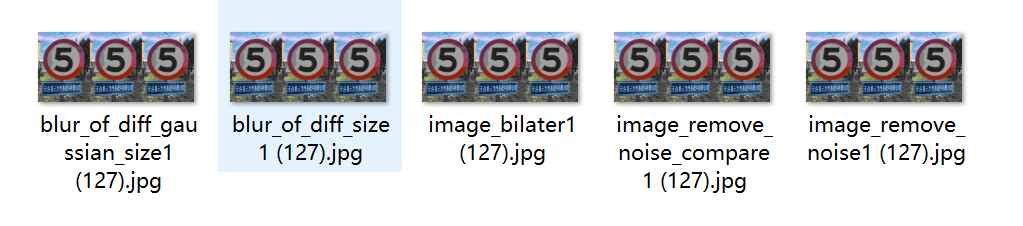
5. Data enhancement:

In the field of deep learning, the requirement for the amount of data is huge. In the field of CV, we enrich the image training set by processing the existing image data through image data enhancement, which can effectively generalize the model and solve the problem of overfitting .

Common image data enhancement methods include rotating images, cropping images, flipping images horizontally or vertically, changing image brightness, etc. In order to facilitate training models, we usually normalize or standardize the data and set the image size to be the same.

6. Code implementation:

There are a few things worth noting in terms of code writing:

1 First, there is a focus layer. For the input image slice, the calculation speed will be faster after reducing the feature map and increasing the channel.

2 Build the model (parse_model) In yolo.py, an array (ch) is used to store the output channels of each layer, and it is easy to form the number of channels output after concatenate during subsequent concatenate.

3 In addition to the last layer of prediction layer, each layer of output channel checks whether it is a multiple of 8 to ensure that there will be no problems in the subsequent concatenation

4 common.py contains various basic blocks, in addition to bottleneck, CSP, concate layers, etc., there are also layers such as transformers.

First import the relevant modules:

import tensorflow as tf
import numpy as np
import pandas as pd 
import cv2
import matplotlib.pyplot as plt
import os
from sklearn.model_selection import train_test_split

Read pictures: The content of target.txt is as follows, the front corresponds to the name of the picture, and the back corresponds to the category of the picture

x=[]
y=[]
with open ('./target.txt','r') as f:
    for j,i in enumerate(f):
        path=i.split()[0]
        lable=i.split()[1]
        print('读取第%d个图片'%j,path,lable)
        src=cv2.imread('./suju/'+path)
        x.append(src)
        y.append(int(lable))

Normalize the data and divide the training set and validation set

x=np.array(x)
y=np.array(y)
x.shape,y.shape
y=y[:,None]
x_train,x_test,y_train,y_test=train_test_split(x,y,stratify=y,random_state=0)
#归一化
x_train=x_train.astype('float32')/255
x_test=x_test.astype('float32')/255

y_train_onehot=tf.keras.utils.to_categorical(y_train)
y_test_onehot=tf.keras.utils.to_categorical(y_test)

Build a network model

model=tf.keras.Sequential([
    tf.keras.Input(shape=(80,80,3)),
    tf.keras.layers.Conv2D(filters=32,kernel_size=(3,3),padding='same',activation='relu'),
    tf.keras.layers.MaxPooling2D(pool_size=(2,2),strides=(2,2)),
    tf.keras.layers.Conv2D(filters=64,kernel_size=(3,3),padding='same',activation='relu'),
    tf.keras.layers.MaxPooling2D(pool_size=(2,2),strides=(2,2)),
    tf.keras.layers.Conv2D(filters=32,kernel_size=(3,3),padding='same',activation='relu'),
    tf.keras.layers.MaxPooling2D(pool_size=(2,2),strides=(2,2)),
    tf.keras.layers.Flatten(),
    tf.keras.layers.Dense(1000,activation='relu'),
    tf.keras.layers.Dropout(rate=0.5),
    tf.keras.layers.Dense(43,activation='softmax')
])
model.compile(
    loss='categorical_crossentropy',
    optimizer='adam',
    metrics=['accuracy']
)
train_history=model.fit(x_train,y_train_onehot,batch_size=100,epochs=8,validation_split=0.2,verbose=1,
          )

Draw a graph to display the loss and acc of the model

la=[str(i) for i in range(1,9)]
def show(a,b,c,d):
    
    
    fig,axes=plt.subplots(1,2,figsize=(10,4))
    axes[0].set_title('accuracy of train and valuation')
    axes[0].plot(la,train_history.history[a],marker='*')
    axes[0].plot(train_history.history[b],marker='*')
    axes[0].set_xlabel('epoch')
    axes[0].set_ylabel('accuracy')
    
    aa=round(train_history.history[a][7],2)
    bb=round(train_history.history[b][7],2)
    
    axes[0].text(la[7],train_history.history[a][7],aa,ha='center',va='bottom')
    axes[0].text(la[7],train_history.history[b][7],bb,ha='center',va='top')
    #axes[0].set_xticks(la,['as','asd',3,4,5,6,7,8])
#     for x1,y1 in zip(la,train_history.history[a]):
#         y1=round(y1,2)
#         axes[0].text(x1,y1,y1,ha='center',va='bottom',fontsize=10,c='b')
        
    axes[0].legend(['train_accuracy','val_accuracy'])
    
    axes[1].set_title('loss of train and valuation')
    axes[1].plot(la,train_history.history[c],marker='*')
    axes[1].plot(train_history.history[d],marker='*')
    axes[1].set_xlabel('epoch')
    axes[1].set_ylabel('loss')
    
    cc=round(train_history.history[c][7],2)
    dd=round(train_history.history[d][7],2)
    
    axes[1].text(la[7],train_history.history[c][7],cc,ha='center',va='top')
    axes[1].text(la[7],train_history.history[d][7],dd,ha='center',va='bottom')
    axes[1].legend(['train_loss', 'val_loss'])
    #axes[1].show()

show('accuracy','val_accuracy','loss','val_loss')

save model

model.save('traffic_model2.h5')

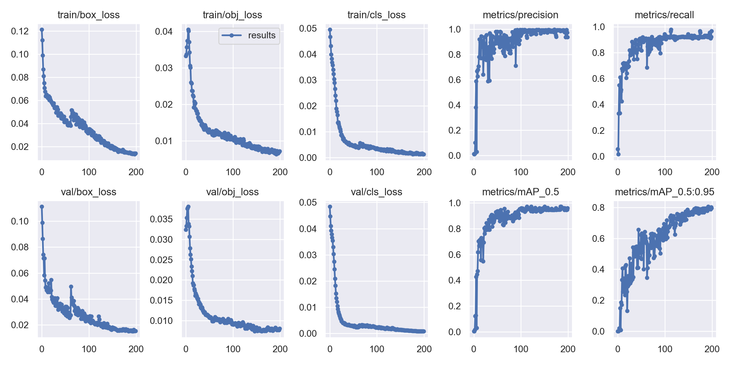
7. Training results:

8. Complete source code & environment deployment video tutorial & data set & custom training video tutorial:

[Administrator deletes, CSDN prohibits free sharing]

9. References:

【1】Xie Dou, Shi Jingwen, Liu Wenjun, Liu Shu. Research on a Traffic Sign Recognition Algorithm Based on Deep Learning[J] . Computer Knowledge and Technology: Academic Edition, 2022,18(6):116-118.
【2】 Wang Zehua, Song Weihu, Wu Jianhua. Lightweight traffic sign detection model based on improved YOLOv4 network[J] . Computer Knowledge and Technology: Academic Edition, 2022,18(5):98-101.