1 Vehicle lateral dynamics model

At high speeds, the orientation of the tires is inconsistent with the direction of the vehicle's speed.
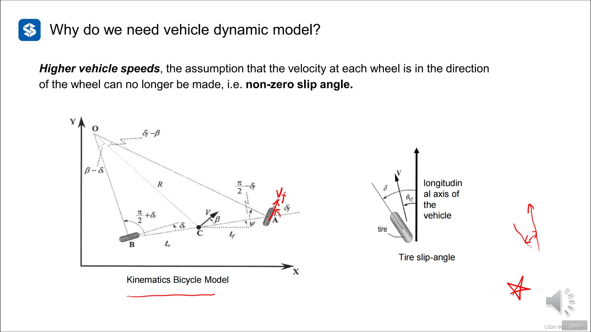

1.1 Lateral Dynamics Modeling
Construct vehicle lateral motion equation, lateral force (force balance), yaw equation (moment balance)
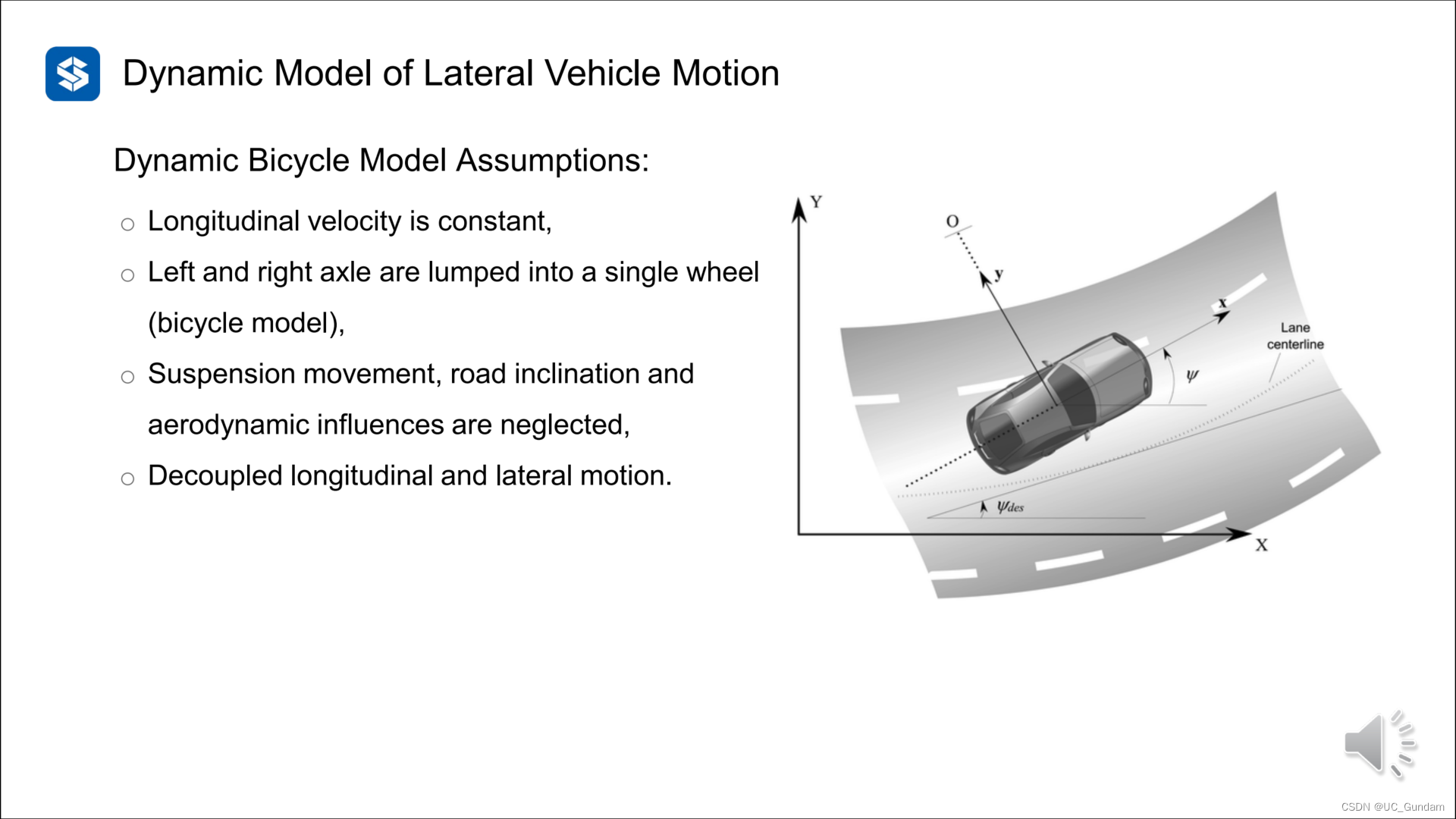
Two degrees of freedom model

Tire lateral force building system
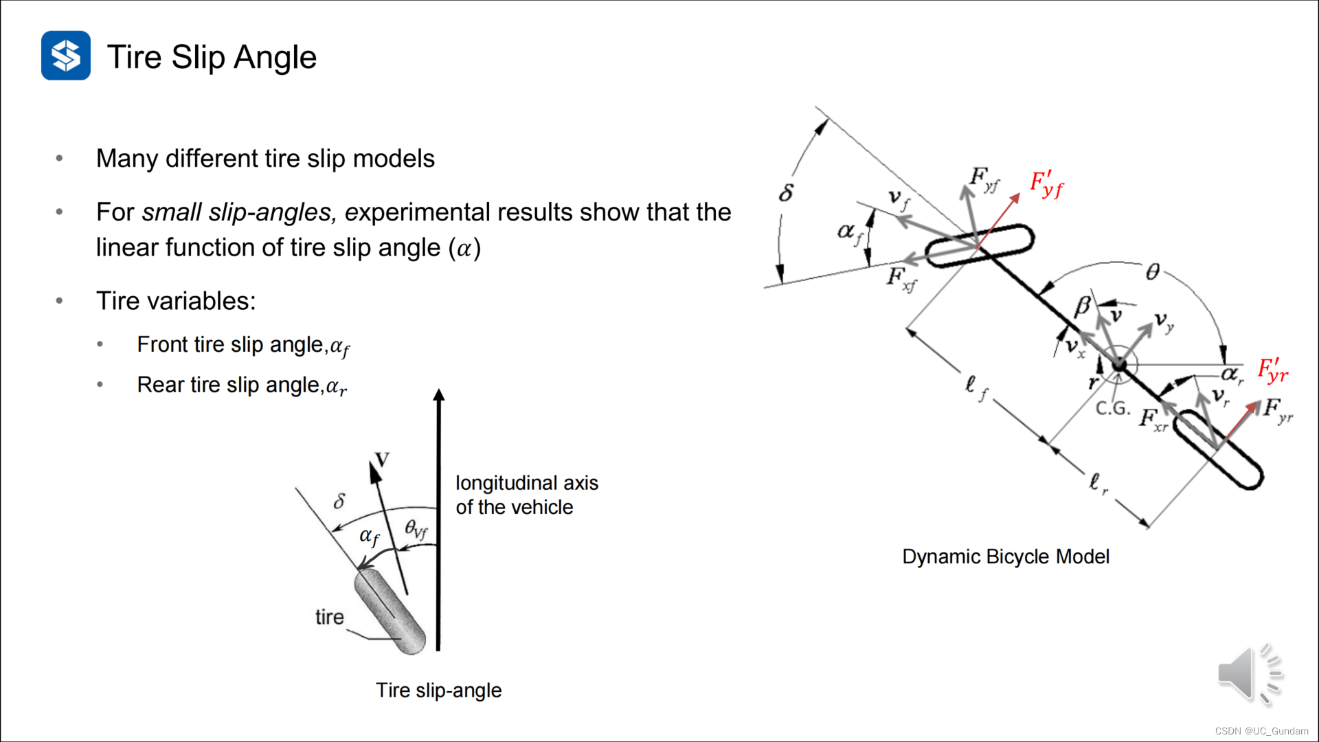
The side slip angle is considered to have a linear relationship with the lateral force, and the slope is the cornering stiffness

Tire lateral force equation, and calculation of wheel deflection (calculated according to the lateral and longitudinal speeds of the vehicle)

Construct the relationship between tire longitudinal force, lateral force and vehicle speed:

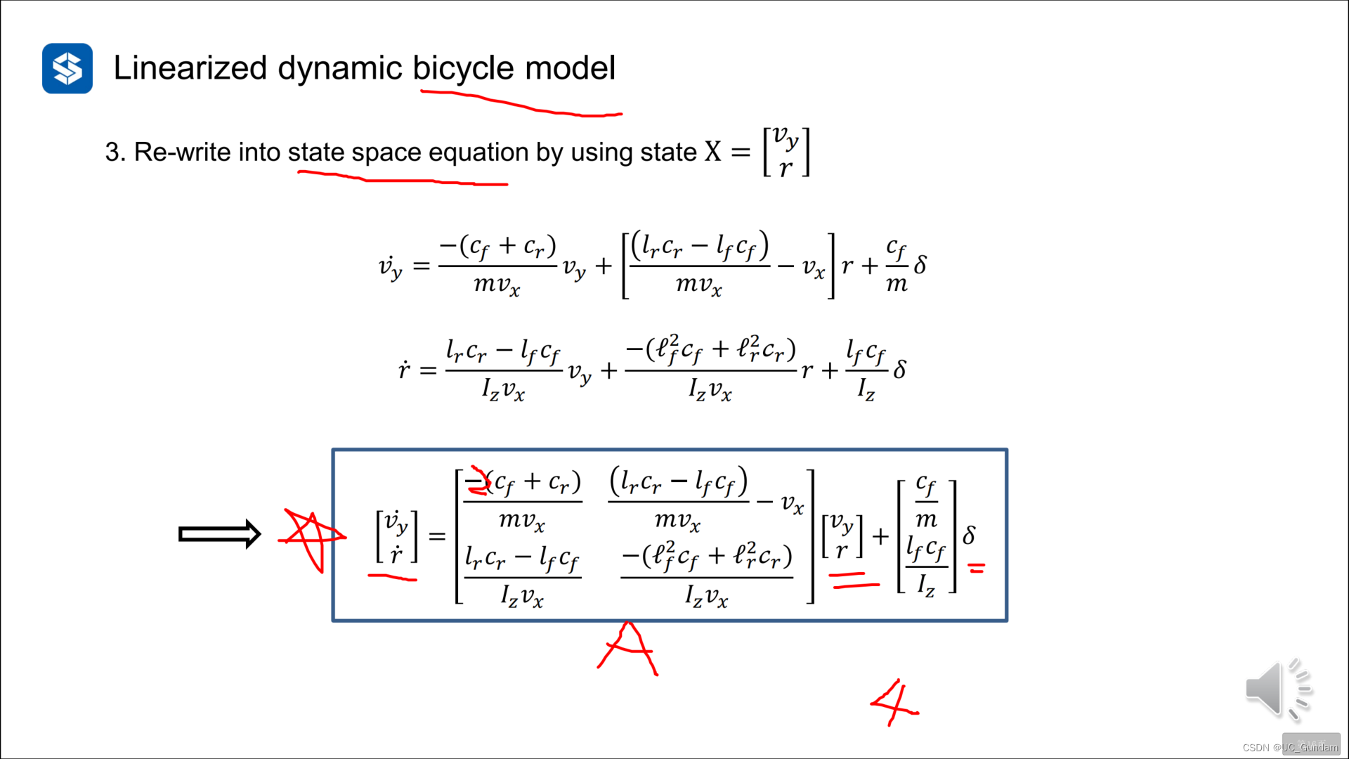
Complete modeling of vehicle lateral dynamics

When applying, adopt certain assumptions to simplify the model:
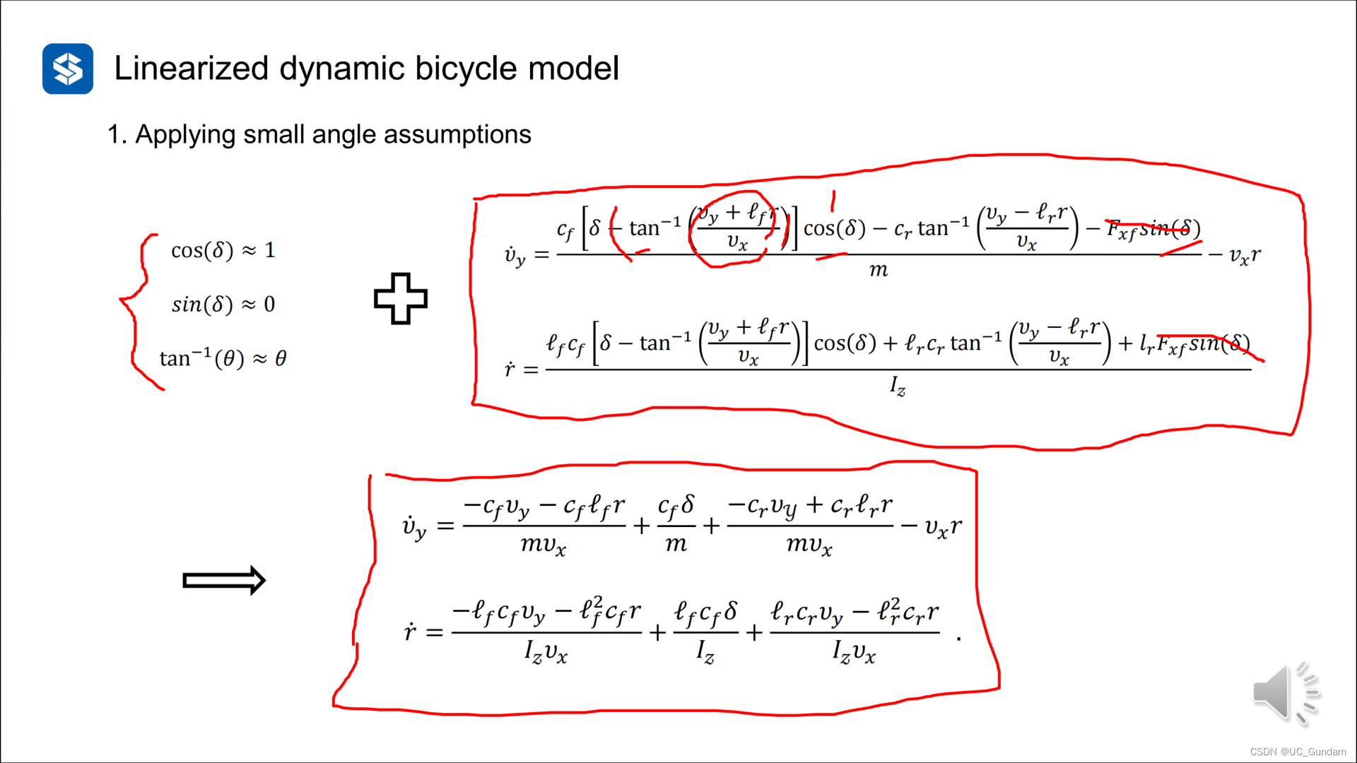

Bicycle model, four-wheel model (add 2 to the coefficient)

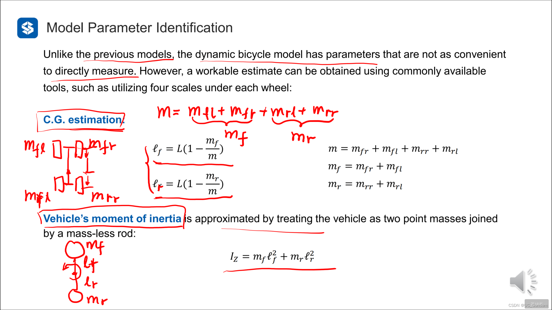
1.2 How to measure important parameters
(1) The position of the center of mass, with four wheels placed on four scales
(2) Moment of inertia, the front and rear wheels have mass and rotate around the center of mass
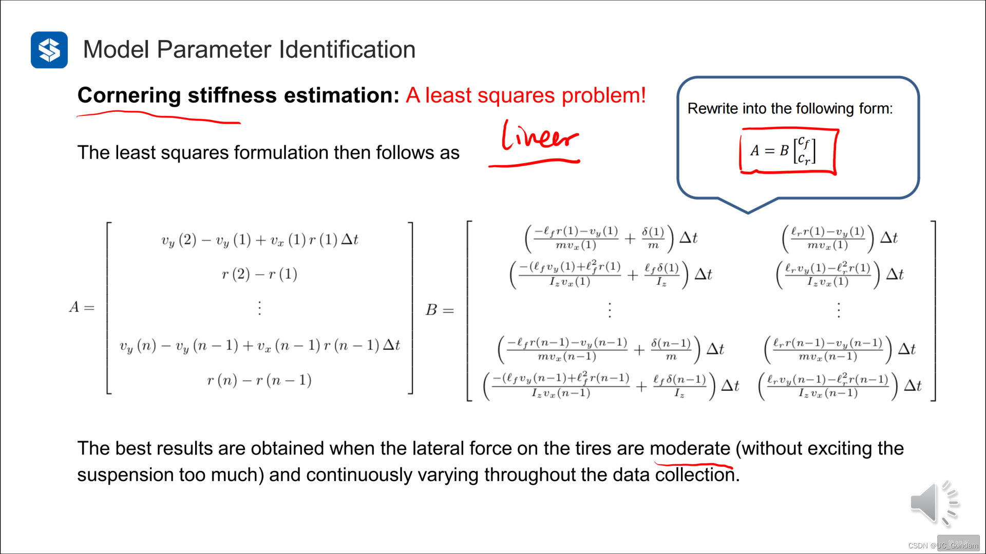
(3) Tire parameters, through experiments, observe the relationship between lateral force and slip angle

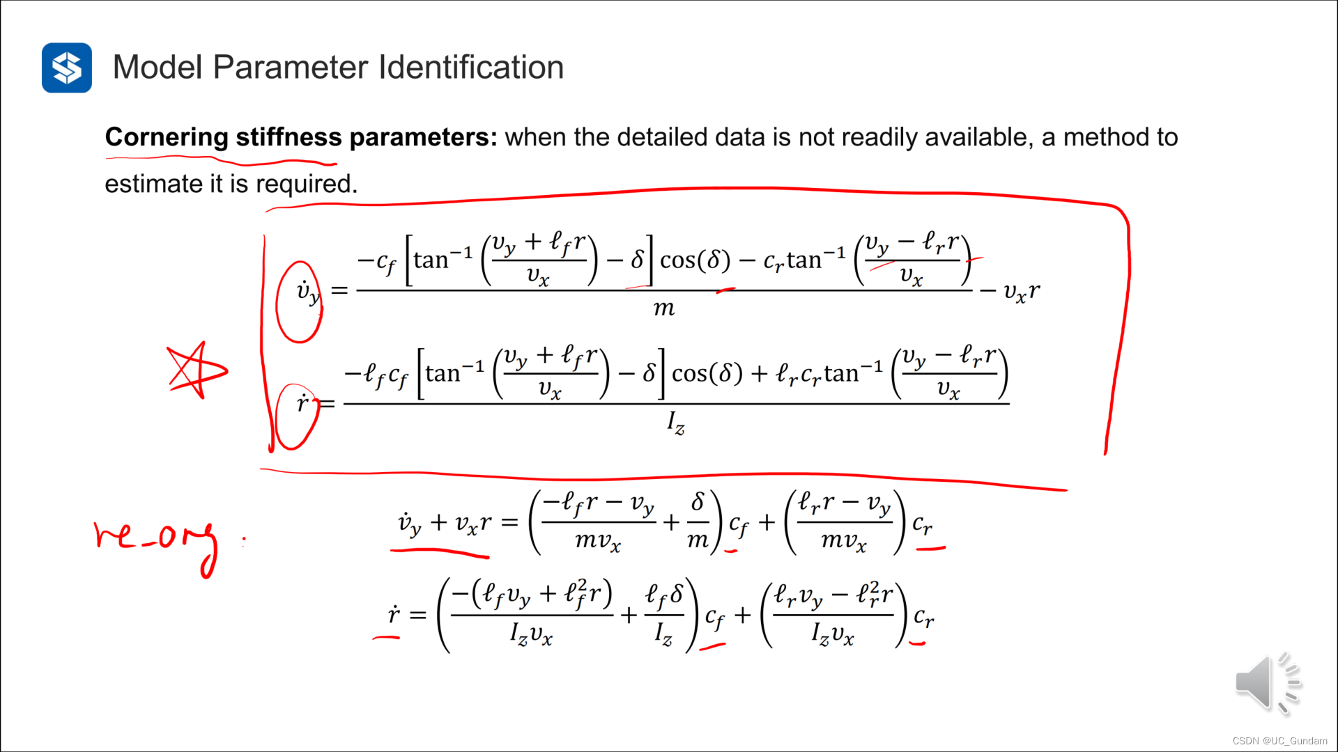
Using the least squares method, more accurate cornering stiffness is calculated.
2 LQR algorithm

2.1 Examples from everyday life
choose travel mode

Quantify choices with weights

For A, time is very important, and the weight of time is very large

For B, money is the most important thing, and money has the greatest weight

The relative value (proportion) of Q and R is the most important, not the absolute value


2.2 for the control system
Control the system to reach the specified position and minimize the cost function
The size of the control variable curve area represents the cost. In order to avoid negative values, the square is used to eliminate it. At the same time, squaring can amplify the error and speed up the convergence.

Q and R are generally expressed in the form of a diagonal matrix, indicating the weight of control parameters and state parameters.

2.2.1 Example of a one-dimensional scalar system
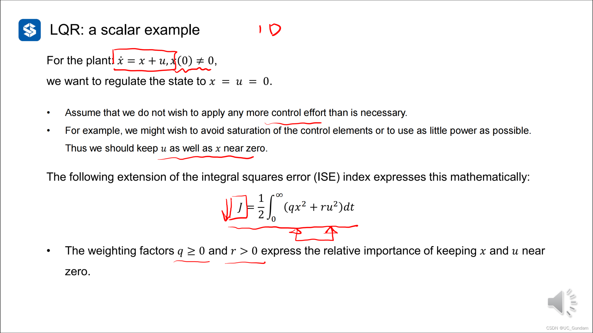
r is 1, only the ratio is considered
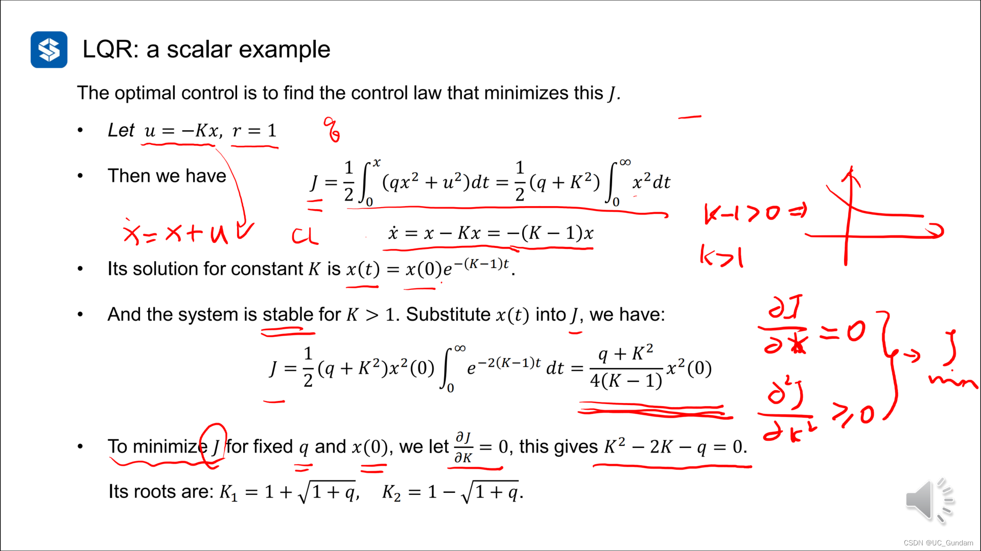

The design of LQR is to choose the Q value and make a trade-off between error and input.
2.2.2 Examples of n-dimensional systems

Introduce P matrix, n×n symmetric matrix
Get the cost function equation

Calculation process of P: eliminate K
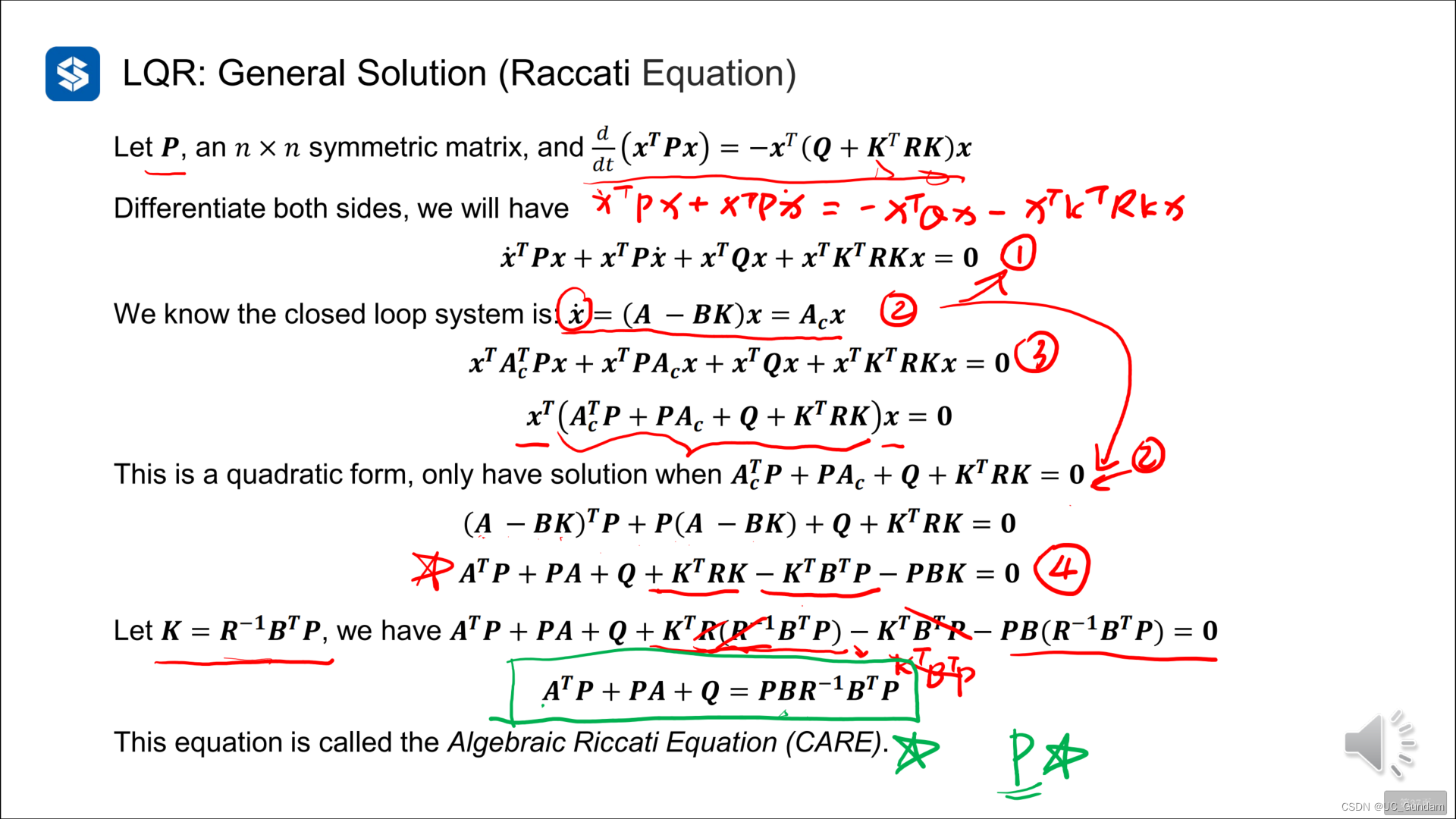
Summarize

2.3 A real example
A mass adjustment system
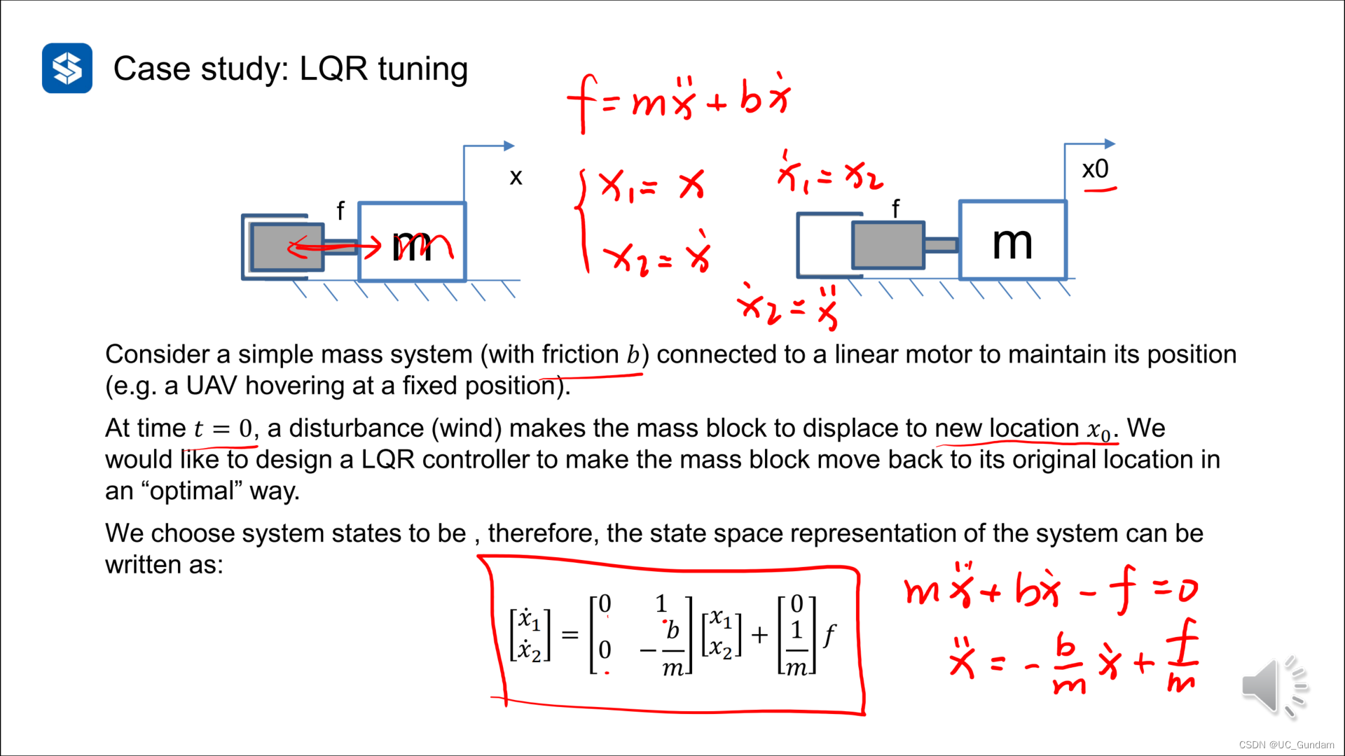

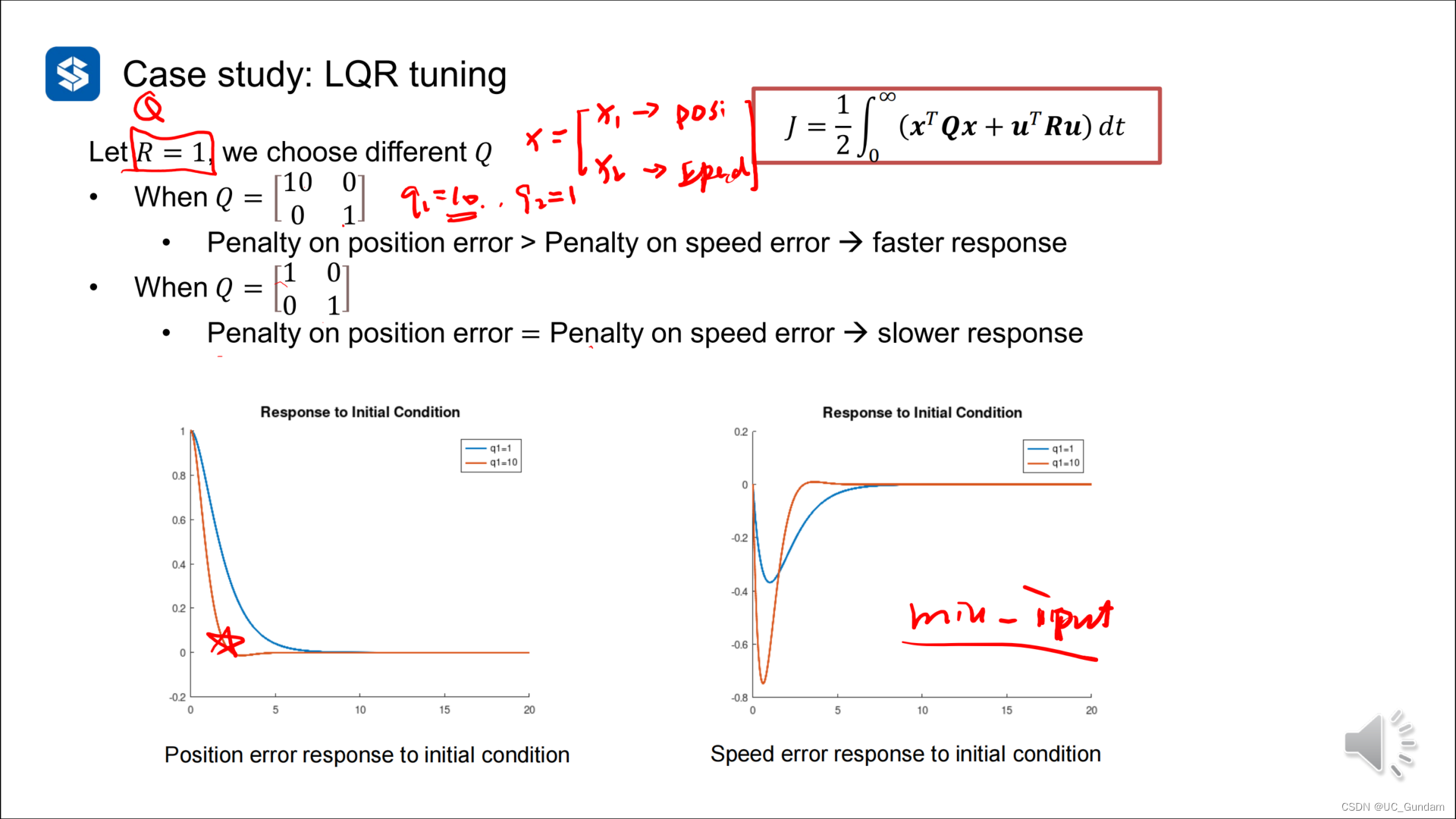
If a faster control effect is required, regardless of the control input, a larger Q value will be selected as much as possible.
If you are very concerned about the input consumption of the controller, the value of R will be optimized first.