Interpretation of YoloV1 paper

Summary

We propose a new approach to object detection: YOLO. Previous work on object detection repurposes classifiers to perform detection. Instead, we treat object detection as a regression problem targeting spatially separated bounding boxes and associated class probabilities. A single neural network can predict bounding boxes and class probabilities directly from full images in a single evaluation. Since the entire detection pipeline is a single network, end-to-end optimization can be directly performed on detection performance.

Our unified architecture is very fast. Our base YOLO model processes images in real time at 45 frames per second. A smaller version of the network, Fast YOLO, processes images at a staggering 155 frames per second, while still achieving twice the mAP of other real-time detectors. Compared with state-of-the-art detection systems, YOLO may make more errors in localization, but is less likely to predict false positives on the background. Finally, YOLO learns very general object representations. It outperforms other detection methods, including DPM and R-CNN, in generalizing from natural images to other domains such as artwork.

1 Introduction

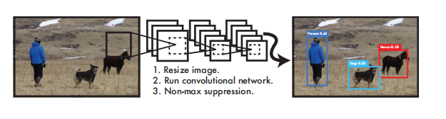
Figure 1: YOLO detection system. Processing images with YOLO is simple and straightforward. Our system (1) resizes the input image to 448×448, (2) runs a convolutional network on the image, and (3) thresholds the detection results by the model's confidence.

Humans can instantly know which objects are in an image, where they are, and how they interact with each other after glancing at an image. The human visual system is fast and accurate, allowing us to perform complex tasks like driving with little awareness of our thinking. Fast and accurate object detection algorithms will enable computers to drive cars without specialized sensors, enable assistive devices to communicate real-time scene information to human users, and unleash the potential of general-purpose, responsive robotic systems.

Current detection systems repurpose classifiers for detection. To detect an object, these systems need to evaluate a classifier for that object at various locations and scales in the test image. Systems like Deformable Part Models (DPM) use a sliding window approach, running the classifier uniformly over the entire image [10]. More recent approaches, such as R-CNN, use region proposal methods to first generate potential bounding boxes in images, and then run classifiers on these proposed bounding boxes. After classification, post-processing is used to refine bounding boxes, remove duplicate detections, and re-score bounding boxes against other objects in the scene [13]. These complex pipelines are slow and hard to optimize because each individual component must be trained separately.

We reformulate object detection as a single regression problem, going directly from image pixels to bounding box coordinates and class probabilities. With our system, you can predict which objects are present in an image and where they are, with just one look at the image. This method is called "you only look once" (YOLO), which is very simple, as shown in Figure 1. A convolutional network simultaneously predicts multiple bounding boxes and class probabilities for those bounding boxes.

YOLO uses full images for training and directly optimizes detection performance. This unified model has several benefits over traditional object detection methods. First, YOLO is very fast. Since we treat detection as a regression problem, complex pipelines are not required. We just need to run our neural network on new images at test time to predict detections. Our base network runs at 45 frames per second on a Titan X GPU, while the fast version runs at over 150 frames per second. This means we can process streaming video in real time with less than 25ms latency. Furthermore, YOLO's average accuracy more than doubles that of other real-time systems. For a live demonstration of our system on a webcam, please see our project webpage: http://pjreddie.com/yolo/.

Second, YOLO considers images globally when making predictions. Unlike sliding window and region proposal-based techniques, YOLO sees the entire image at both training and test time, thus implicitly encoding contextual information about categories and their appearance. A state-of-the-art detection method, Fast R-CNN, mistook background regions in an image for objects due to its inability to see the larger context. In contrast, YOLO has less than half the background error.

Third, YOLO learns a generalizable representation of objects. When trained on natural images and tested on artwork, YOLO outperforms top detection methods like DPM and R-CNN. Since YOLO is highly generalizable, it is less likely to fail when applied to new domains or unexpected inputs.

YOLO still lags behind state-of-the-art detection systems in accuracy. While it can quickly identify objects in images, it struggles to pinpoint some objects, especially small ones. We explore these tradeoffs further in our experiments.

2. Unified detection

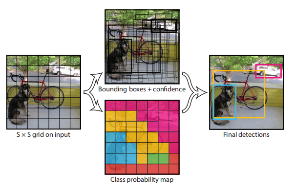
Figure 2: Model. Our system models detection as a regression problem. It partitions the image into an S×S grid and predicts B bounding boxes, confidences for these boxes, and class C probabilities for each grid cell. These predictions are encoded as a $S \times S \times （ B * 5 + C)$ Tensors.

We unify the various components of object detection into a single neural network. Our network uses features from the entire image to predict each bounding box. It also predicts all bounding boxes for all classes in the image simultaneously. This means that our network makes global inferences about the entire image and all objects in the image. YOLO is designed so that we can train it end-to-end and achieve real-time speed while maintaining high average accuracy.

Our system divides the input image into an $S \times S$ grid. If the center of an object falls into a grid cell, then that grid cell is responsible for detecting the object.

Each grid cell predicts $B$ bounding boxes and corresponding confidence scores. These confidence scores reflect how confident the model thinks that the box contains an object and how accurately it predicts the box. We formally define the confidence as $Pr(Object)∗IOU^{truth}_{pred}$ . If no object exists in that cell, the confidence score should be zero. Otherwise, we want the confidence score to be equal to the IOU (intersection over union) between the predicted box and the actual box.

Each bounding box consists of 5 predictions: $x, y, w, h$ and confidence. where $The (x, y)$ coordinates represent the center of the bounding box relative to the grid cell. Width and height are predicted relative to the entire image. Finally, the confidence prediction represents the IOU between the predicted box and any ground-truth box.

Each grid cell also predicts C conditional class probabilities, $Pr(Class_i|Object)$ . These probabilities are predicted conditioned on the grid cell containing an object. We predict only one set of class probabilities per grid cell, regardless of the number B of bounding boxes.

At test time, we multiply the conditional class probabilities and individual box confidence predictions

$Pr(Class_i|Object)*Pr(Object)*IOU^{truth}_{pred}=Pr(Class_i)*IOU^{truth}_{pred} (1)$

This gives us a category-specific confidence score for each box. These scores encode both the probability that the class appears in the box and how well the predicted box matches the object.

We use S = 7, B = 2 when evaluating YOLO on the PASCAL VOC dataset. The PASCAL VOC dataset has 20 labeled categories, so C = 20. Our final prediction is a 7x7x30 tensor.

2.1 Network Design

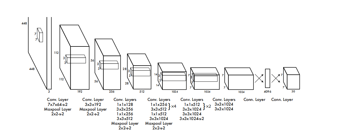
Figure 3: Network structure. Our detection network consists of 24 convolutional layers and 2 fully connected layers. Alternately used 1×1 convolutional layers can reduce the feature space of the previous layers. We pre-train convolutional layers at half-resolution (224×224 input images) on the ImageNet classification task, and then double the resolution for detection.

We implement this model as a convolutional neural network and evaluate it on the PASCAL VOC detection dataset [9]. The initial convolutional layers of the network extract features from the image, while the fully connected layers predict the probabilities and coordinates of the outputs.

Our network architecture is inspired by the GoogLeNet image classification model [34]. Our network consists of 24 convolutional layers and 2 fully connected layers. Instead of using the Inception module in GoogLeNet, we employ a 1×1 dimensionality reduction layer followed by a 3×3 convolutional layer, similar to the method of Lin et al. [22]. The complete network structure is shown in Figure 3.

We also train a fast version of YOLO designed to push the boundaries of fast object detection. Fast YOLO uses fewer convolutional layers (only 9 instead of 24) and fewer filters. All training and testing parameters are the same between YOLO and Fast YOLO except the network size.

The final output of our network is a 7×7×30 prediction tensor.

2.2 Training

We pre-train our convolutional layers on the ImageNet 1000-class competition dataset [30]. For pre-training, we use the first 20 convolutional layers in Figure 3, followed by an average pooling layer and a fully connected layer. We train this network for about a week and achieve a single crop top-5 accuracy of 88% on the ImageNet 2012 validation set, comparable to the GoogLeNet model in the Caffe model library [24]. We use the Darknet framework for all training and inference [26].

Then, we convert the model to perform detection. Ren et al. showed that adding convolutional and connection layers to a pretrained network can improve performance [29]. Following their example, we added four convolutional layers and two fully connected layers with weights initialized randomly. Detection usually requires fine-grained visual information, so we increase the input resolution of the network from 224 × 224 to 448 × 448.

Our last layer predicts class probabilities and bounding box coordinates. We normalize the bounding box width and height by the image width and height so that they fall between 0 and 1. We parameterize the bounding box x and y coordinates as offsets from specific grid cell locations, so they are also constrained between 0 and 1.

We use a linear activation function in the last layer and the following rectified linear activation function in all other layers:

$\begin{cases} 0.1x, & x <= 0 \\ x, & otherwise \end{cases}(2)$

The optimization objective for our model output is the sum-squared error. We use total mean squared error because it is easy to optimize, however it does not quite fit our goal of maximizing average precision. It weighs localization error and classification error equally , which may not be ideal. Also, in each image, many grid cells do not contain any objects. This drives the "confidence" scores of these cells towards zero, tending to overwhelm the gradient of cells containing objects. This can lead to model instability, making training diverge prematurely.

To address this, we increase the loss for bounding box coordinate predictions and decrease the loss for bounding box confidence predictions that do not contain objects. We used two parameters $λ_{coord}$ 和 $λ_{noobj}$ to achieve this. We will $λ_{coord}$ Set to 5, the $λ_{noobj}$ Set to 0.5.

The total mean squared error weighs the errors in the large and small boxes equally. Our error metric should reflect the different importance of small deviations in large and small boxes. To partially address this problem, we predict the square root of the bounding box width and height instead of predicting the width and height directly.

YOLO predicts multiple bounding boxes per grid cell. At training time, we only want one bounding box predictor to be responsible for each object prediction. We assign a predictor to be "responsible" for predicting an object based on the current prediction with the highest IOU compared to the ground truth. This leads to specialization among bounding box predictors. Each predictor becomes more accurate at predicting objects of a specific size, aspect ratio, or class, improving overall recall.

During training, we optimize the following multipart loss function:

$\lambda_{coord}\sum^{S^2}_{i=0}\sum^{B}_{j=0}1^{obj}_{ij}[(x_i-\hat{x}_i)^2+(y_i-\hat{y}_i)^2]\\+\lambda_{coord}\sum^{S^2}_{i=0}\sum^{B}_{j=0}1^{obj}_{ij}[(\sqrt{w_i}-\sqrt{\hat{w}_i})^2+(\sqrt{h_i}-\sqrt{\hat{h}_i})^2] \\ +\sum^{S^2}_{i=0}\sum^{B}_{j=0}1^{obj}_{ij}(C_i-\hat{C_i})^2\\ + \lambda_{noojb}\sum^{S^2}_{i=0}\sum^{B}_{j=0}1^{noobj}_{ij}(C_i-\hat{C_i})^2\\+\sum^{S^2}_{i=0}1^{obj}_{i}\sum_{c\in classes}(p_i(c)-\hat{p_i}(c))^2(3)$

Among them, $1^{obj}_{ij}$ Indicates whether the object appears in the $i $th cell, $1^{obj}_{ij}$ Indicates the th cell in the th cell in the $i The j$th bounding box predictor $in cell "responsible" for that prediction.$

Note that the loss function penalizes classification error (hence the conditional class probabilities discussed earlier) only when there is an object in the grid cell. It only penalizes bounding box coordinate errors if that predictor is "in charge" of the ground truth box (i.e. the predictor with the highest IOU in that grid cell).

We train the network for about 135 epochs on the PASCAL VOC 2007 and 2012 training and validation datasets. When testing against 2012, we also include the test data of VOC 2007 for training. Throughout training, we use a batch size of 64, a momentum of 0.9 and a decay rate of 0.0005.

Our learning rate schedule is as follows: Over the first few epochs, we slowly increase the learning rate from 10^(-3) to 10^(-2). If we start with a high learning rate, the model tends to diverge due to unstable gradients. We continue with 10^(-2) for 75 epochs, then 10^(-3) for 30 epochs, and finally 10^(-4) for 30 epochs.

To avoid overfitting, we use dropout and extensive data augmentation. After the first connection layer, the dropout layer has a rate of 0.5 to prevent co-adaptation between layers [18]. For data augmentation, we introduce random scaling and translation up to 20% of the original image size. We also randomly adjust the exposure and saturation of images in HSV color space by up to a factor of 1.5.

2.3 Reasoning

Just like in training, predicting detections in test images requires only one network evaluation. On PASCAL VOC, the network predicts 98 bounding boxes per image and a class probability for each box. Since it requires only one network evaluation, YOLO is very fast at test time, unlike classifier-based methods.

The grid design enforces spatial diversity in bounding box predictions. Typically, it is possible to determine which grid cell an object belongs to, so the network only predicts one box per object. However, some large objects or objects close to the boundaries of multiple cells can be well localized by multiple cells. Non-maximum suppression can be used to fix these multiple detections. While as critical as R-CNN or DPM, non-maximum suppression can increase mAP by 2-3%.

2.4. Limitations of YOLO

YOLO imposes strong spatial constraints on bounding box predictions, since each grid cell only predicts two boxes and can only have one class. This spatial constraint limits the number of nearby objects the model can predict. Our model has difficulty recognizing small objects that appear in groups, such as a flock of birds.

Since our model learns to predict bounding boxes from data, it has difficulty generalizing to objects with new or unusual aspect ratios or configurations. Our model also uses relatively coarse features to predict bounding boxes because our architecture has multiple downsampling layers from the input image.

Finally, while our trained loss function approximates detection performance, our loss function handles errors equally in small and large bounding boxes. Small errors in large boxes are usually harmless, but small errors in small boxes have a larger impact on IOU. Our main source of error is wrong positioning.

3. Comparison with other object detection frameworks

Object detection is a central problem in computer vision. Detection pipelines usually extract a robust set of features (such as Haar [25], SIFT [23], HOG [4], convolutional features [6]) from the input image, and then use classifiers [36, 21, 13, 10 ] or localizers [1, 32] to identify objects in feature space. These classifiers or localizers operate in a sliding-window fashion over the entire image, or on a subset of certain regions of the image [35, 15, 39]. We compare the YOLO detection system to several top detection frameworks, highlighting key similarities and differences.

Deformable Part Model (DPM)

DPM uses a sliding window approach for object detection [10]. DPM uses disjoint pipelines to extract static features, classify regions, predict bounding boxes for high-scoring regions, and more. Our system replaces all these disparate parts with a single convolutional neural network. The network performs feature extraction, bounding box prediction, non-maximum suppression, and contextual inference, all simultaneously. Instead of using static features, the network trains feature lines and optimizes them for the detection task. Our unified architecture is faster and more accurate than DPM.

R-CNN

R-CNN and its variants use region proposals instead of sliding windows to find objects in images. Selective Search [35] generates potential bounding boxes, convolutional network extracts features, SVM scores boxes, linear model adjusts bounding boxes, and non-maximum suppression eliminates duplicate detections. Each stage of this complex process had to be adjusted precisely and independently, and as a result the system was very slow, taking more than 40 seconds per image when tested.

YOLO shares some similarities with R-CNN. Each grid cell proposes potential bounding boxes, and convolutional features are used to score these boxes. However, our system imposes spatial constraints on grid cell proposals that help alleviate multiple detections of the same object. Our system also proposes far fewer bounding boxes than Selective Search, only 98 per image. Finally, our system merges these individual components into a unified optimized model.

Other rapid detectors

Fast and Faster R-CNN focus on increasing the speed of R-CNN by sharing computation and using neural network instead of Selective Search [14][28]. Although they have improved over R-CNN in terms of speed and accuracy, they still cannot achieve real-time performance. Many research works focus on accelerating DPM pipelines [31][38][5]. They accelerate HOG calculations, use cascades and push calculations to the GPU. However, only 30Hz DPM [31] can actually run in real time. Unlike optimizing individual components of a large detection pipeline, YOLO completely abandons the pipeline and achieves fast detection by design.

Single-class detectors, such as face or human shape detectors, can be highly optimized because they need to deal with a smaller range of variation [37]. YOLO is a general purpose detector that learns to detect various objects simultaneously.

Deep MultiBox

Unlike R-CNN, Szegedy et al. train a convolutional neural network to predict regions of interest [8] instead of using Selective Search. MultiBox can also perform single object detection by replacing confidence predictions with single class predictions. However, MultiBox cannot perform general object detection and is still only a part in a larger detection pipeline, requiring further image patch classification. Both YOLO and MultiBox use convolutional networks to predict bounding boxes in images, but YOLO is a complete detection system.

OverFeat

Sermanet et al. trained a convolutional neural network to perform localization and adapted the localizer to perform detection [32]. OverFeat efficiently performs sliding window detection, but is still a disjoint system. OverFeat optimizes localization rather than detection performance. Like DPM, the locator only sees local information when making predictions. OverFeat cannot reason about the global context, so extensive post-processing is required to produce coherent detection results.

MultiGrasp

Our design is similar to the work of Redmon et al. [27] on grasp detection. Our grid approach to bounding box prediction is based on the MultiGrasp system for regression to grasped regions. However, grasp detection is much simpler than object detection. MultiGrasp only needs to predict a graspable region for an image containing an object. It does not need to estimate an object's size, location, or boundary, nor predict its class, only to find a suitable region for grasping. YOLO predicts bounding boxes and class probabilities for multiple objects of multiple classes in an image.

4. Experiment

We first compare YOLO with other real-time detection systems on PASCAL VOC 2007. To understand the differences between YOLO and R-CNN variants, we explore the errors of YOLO and Fast R-CNN on VOC 2007. Fast R-CNN is one of the highest performance versions of R-CNN [14]. Based on different error profiles, we show that YOLO can be used to re-score Fast R-CNN detection results and reduce background false positive errors, leading to significant performance improvements. We also show results on VOC 2012 and compare the average accuracy with current state-of-the-art methods. Finally, we show that YOLO generalizes better than other detectors on two artwork datasets.

4.1. Comparison with other real-time systems

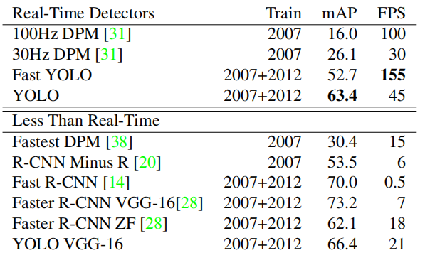
Table 1: Real-time systems on PASCAL VOC 2007. Compare the performance and speed of the fast detectors. Fast YOLO is the fastest detector on record for PASCAL VOC detection, still more than two times more accurate than any other real-time detector. YOLO is 10 mAP more accurate than the fast version, while still being much faster than real-time.

Much research on object detection focuses on improving the speed of standard detection pipelines. [5] [38] [31] [14] [17] [28] However, only Sadeghi et al. have actually implemented a detection system that runs in real time (30 frames per second or faster) [31]. We compare YOLO to their GPU-implemented DPM, which can run at 30Hz or 100Hz. Although other studies have not reached the real-time milestone, we still compare their relative mAP and speed to investigate the accuracy-performance trade-off available in object detection systems.

Fast YOLO is the fastest object detection method on PASCAL; to our knowledge, it is the fastest existing object detector. With a mAP of 52.7%, it more than doubles the accuracy of previous work for real-time detection. YOLO pushes mAP to 63.4%, while still maintaining real-time performance.

We also train YOLO using VGG-16. This model is more accurate but much slower than YOLO. It is useful for comparison with other detection systems that rely on VGG-16, but since it is slower than real-time, the rest of this paper focuses on our faster model.

Fastest DPM effectively speeds up DPM without sacrificing too much mAP, but it is still two times slower relative to real-time performance [38]. It is also limited by the relatively low accuracy of DPM in detection, compared to neural network approaches.

R-CNN minus R replaces selective search [20] with static bounding box proposals. Although it is much faster than R-CNN, it still cannot reach real-time, and the accuracy suffers significantly due to the lack of good proposals.

Fast R-CNN speeds up the classification stage of R-CNN, but it still relies on selective search and takes about 2 seconds per image to generate bounding box proposals. So it has high mAP, but is far from realtime at 0.5 fps.

The recent Faster R-CNN uses a neural network to propose bounding boxes, similar to Szegedy et al. [8]. Their most accurate model achieved 7 fps in our tests, while the smaller but less accurate model ran at 18 fps. The VGG-16 version of Faster R-CNN is 10 mAP lower than YOLO, but 6 times slower than YOLO. Zeiler-Fergus Faster R-CNN is 2.5 times slower than YOLO, but less accurate.

4.2. VOC 2007 error analysis

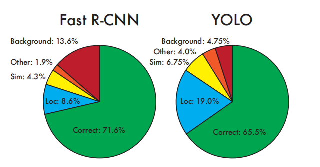
Figure 4: Error Analysis: Fast R-CNN vs. YOLO. These graphs show the percentage of localization errors and background errors in the top N detections for each class (N = number of objects in that class).

To further investigate the differences between YOLO and state-of-the-art detectors, we looked at the detailed analysis of results on VOC 2007. We compare YOLO with Fast R-CNN because Fast R-CNN is one of the best performing detectors on PASCAL and its detection results are publicly available.

We use the method and tools of Hoiem et al. [19]. At test time, for each class, we look at the top N predictions for that class. Each prediction can be correct or classified according to the type of error:

• Correct: correct class and IOU > .5
• Localization: correct class, .1 < IOU < .5
• Similar: similar class, IOU > .1
• Other: wrong class, IOU > .1
• Background: any object IOU < .1

Figure 4 shows the average breakdown of each error type across all 20 categories.

YOLO has difficulty locating objects correctly. Localization errors make up the majority of YOLO's errors, more than all other sources of errors combined. Fast R-CNN has far fewer localization errors than YOLO, but much more background errors. 13.6% of its top-N detections are false positives that do not contain any objects. Fast R-CNN is nearly three times more likely to predict background detection results than YOLO.

4.3. Combining Fast R-CNN and YOLO

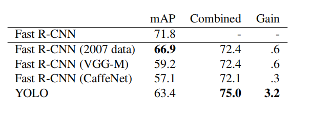
Table 2: Model combination experiments on VOC 2007. We study the effect of combining various models with the best version of Fast R-CNN. Other versions of Fast R-CNN provide only marginal benefits, while YOLO can significantly improve performance.

YOLO makes fewer background errors than Fast R-CNN. By using YOLO to eliminate the background detection results of Fast R-CNN, we can significantly improve the performance. For each bounding box predicted by R-CNN, we check whether there is a similar bounding box predicted by YOLO. If it does, we give YOLO a bonus to that prediction based on its predicted probability and the overlap between the two bounding boxes.

The best Fast R-CNN model achieves 71.8% mAP on the VOC 2007 test set. When combined with YOLO, its mAP increased by 3.2% to 75.0%. We also try to combine the best Fast R-CNN model with several other Fast R-CNN versions. These ensembles produced small increases between 0.3% and 0.6%, as detailed in Table 2.

The improvement in YOLO is not just a by-product of model ensembles, as there is little benefit in combining different versions of Fast R-CNN. On the contrary, precisely because YOLO makes different types of mistakes at test time, it is very effective in improving the performance of Fast R-CNN.

Unfortunately, this combination does not benefit from the speed of YOLO because we run each model separately and then combine the results. However, since YOLO is very fast, it does not add any significant computation time compared to Fast R-CNN.

4.4. VOC 2012 Results

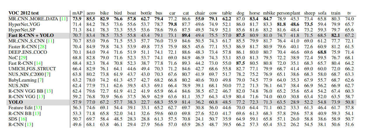
Table 3: PASCAL VOC 2012 leaderboard. As of November 6, 2015, YOLO was compared to the full comp4 public leaderboard that allows the use of external data. The average precision of various detection methods and the average precision per class are shown. YOLO is the only real-time detector. Fast R-CNN + YOLO is the fourth highest scoring method, improving by 2.3% over Fast R-CNN.

4.5. Generality: Person Detection in Artwork

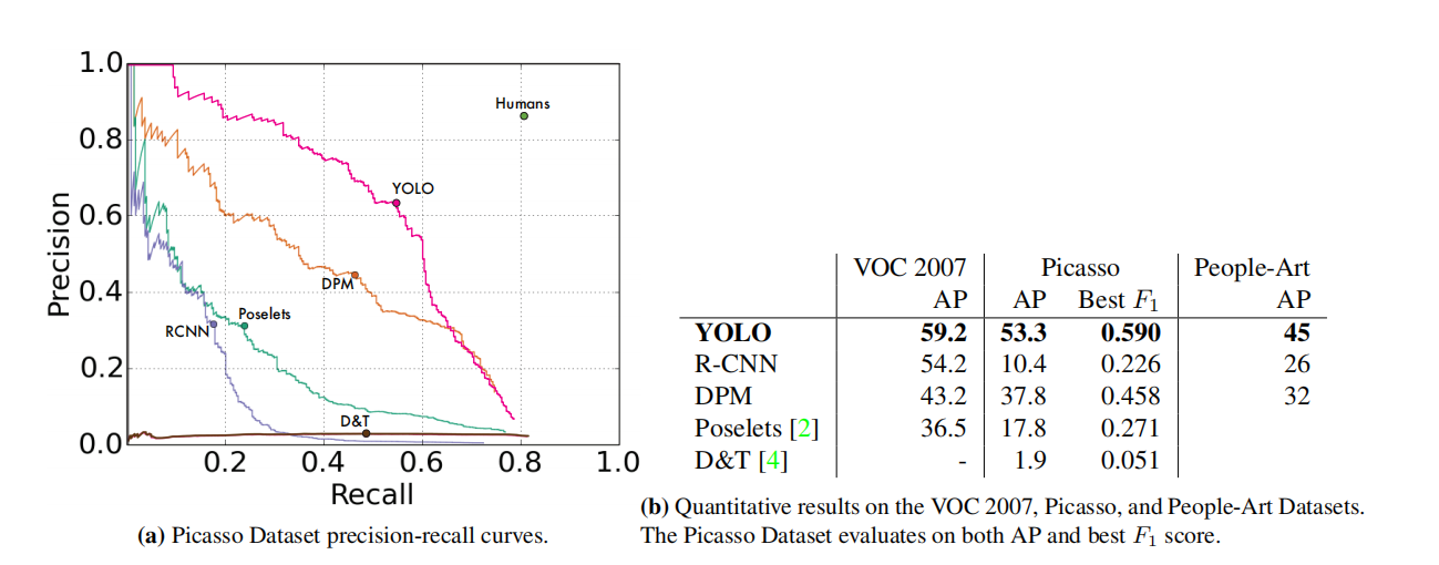
Figure 5: Generalizability results on Picasso and People-Art datasets.

Academic datasets for object detection draw training and test data from the same distribution. In practical applications, it is difficult to predict all possible use cases, and the test data may be different from what the system has seen before [3]. We compare YOLO to other detection systems on the Picasso dataset [12] and the People-Art dataset [3], which are used to test detection of people in artworks.

Figure 5 shows the comparative performance between YOLO and other detection methods. For reference, we present the VOC 2007 detection AP on people when all models are trained on VOC 2007 data only. On Picasso, the model is trained on VOC 2012, while on People-Art, the model is trained on VOC 2010.

On VOC 2007, R-CNN has a higher AP. However, when applied to artworks, the performance of R-CNN drops significantly. R-CNN uses selective search to propose bounding boxes, which works well for natural images. The classifier in R-CNN only looks at small regions and requires good proposals.

DPM maintains its AP level when applied to artwork. Previous work theorized that DPM performs well because it has a strong spatial model of object shape and layout. Although DPM is not as degenerate as R-CNN, it has a lower starting point.

YOLO has good performance on VOC 2007 and its AP drops less than other methods when applied to artworks. Similar to DPM, YOLO simulates the size and shape of objects, as well as the relationship between objects and where objects usually appear. Although artwork and natural images are very different at the pixel level, they are similar in terms of object size and shape, so YOLO can still predict good bounding boxes and detection results.

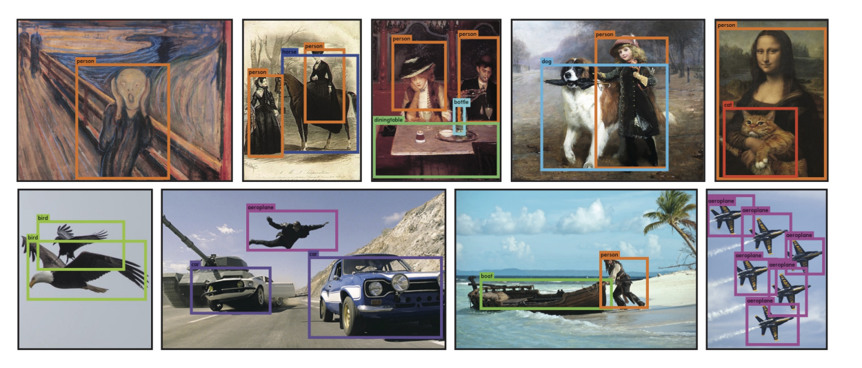
Figure 6: Qualitative results. YOLO runs on sample artwork and nature images from the internet. While it does think a person is an airplane, it's mostly accurate

5. Real-time detection in the wild

YOLO is a fast and accurate object detector ideal for computer vision applications. We hooked up YOLO to a webcam and verified that it maintains real-time performance, including the time it takes to acquire images from the camera and display detection results.

The resulting system is interactive and engaging. While YOLO processes each image individually, when connected to a webcam it works like a tracking system, detecting object movement and changes in appearance. A demo and source code of the system is available on our project website: http://pjreddie.com/yolo/.

6 Conclusion

We introduce YOLO, a unified model for object detection. Our model is simple to build and can be trained directly on full images. Unlike classifier-based methods, YOLO is trained on a loss function that directly corresponds to detection performance, and the entire model is jointly trained.

Fast YOLO is the fastest general-purpose object detector in the literature, and YOLO pushes the state-of-the-art in real-time object detection. YOLO also generalizes well to new domains, making it ideal for applications that rely on fast, robust object detection.

code explanation

The code in this article comes from: code , intrusion and deletion

Project structure:

Read XML file information (write_txt.py)
Dataset preprocessing (yoloData.py)
YOLOV1 network structure definition (resnet50.py)
Loss function definition (yoloLoss.py)
Train the network (train.py)
make predictions (predict.py)

write_txt.py

VOC format

First introduce the VOC data format:

VOC (Visual Object Classes) data format is a widely used data format, mainly used in computer vision tasks such as image classification, object detection and segmentation. It originated from the PASCAL VOC (Pattern Analysis, Statistical Modeling and Computational Learning Visual Object Classes) challenge, a computer vision competition held between 2005-2012.

The VOC data format consists of two parts: image data and annotation data.

Image data: Stores image files, usually in JPG format.
Annotation data: store annotation information related to images, usually XML files. Annotation information for each image is in a separate XML file. The XML file follows the following structure:

<annotation>
    <folder>图像所在文件夹名称</folder>
    <filename>图像文件名</filename>
    <source>
        <database>图像来源数据库</database>
        <annotation>标注来源</annotation>
        <image>图像来源</image>
    </source>
    <size>
        <width>图像宽度</width>
        <height>图像高度</height>
        <depth>图像通道数</depth>
    </size>
    <segmented>是否用于分割任务(0或1)</segmented>
    <object>
        <name>物体类别名称</name>
        <pose>物体姿态</pose>
        <truncated>物体是否被截断(0或1)</truncated>
        <difficult>物体是否难以识别(0或1)</difficult>
        <bndbox>
            <xmin>边界框左上角 x 坐标</xmin>
            <ymin>边界框左上角 y 坐标</ymin>
            <xmax>边界框右下角 x 坐标</xmax>
            <ymax>边界框右下角 y 坐标</ymax>
        </bndbox>
    </object>
    ...
</annotation>

The main advantage of the VOC data format is that it is simple to understand and easy to parse. However, with the development of the field of deep learning and computer vision, new data formats (such as COCO and YOLO) have emerged and are widely used, and they have higher flexibility and efficiency in some aspects. Nonetheless, the VOC data format remains a fundamental data format in the field of computer vision.

the code

Guide package

import xml.etree.ElementTree as ET
import os
import random

define class

VOC_CLASSES = (  # 定义所有的类名
    'aeroplane', 'bicycle', 'bird', 'boat',
    'bottle', 'bus', 'car', 'cat', 'chair',
    'cow', 'diningtable', 'dog', 'horse',
    'motorbike', 'person', 'pottedplant',
    'sheep', 'sofa', 'train', 'tvmonitor')  # 使用其他训练集需要更改

define path

train_set = open('voctrain.txt', 'w')
test_set = open('voctest.txt', 'w')
Annotations = 'VOCdevkit//VOC2007//Annotations//'

split dataset test set

xml_files = os.listdir(Annotations)
random.shuffle(xml_files)  # 打乱数据集
train_num = int(len(xml_files) * 0.7)  # 训练集数量
train_lists = xml_files[:train_num]  # 训练列表
test_lists = xml_files[train_num:]  # 测测试列表

parse xml file

def parse_rec(filename):  # 输入xml文件名
    tree = ET.parse(filename)
    objects = []
    # 查找xml文件中所有object元素
    for obj in tree.findall('object'):
        # 定义一个字典，存储对象名称和边界信息
        obj_struct = {
    
    }
        difficult = int(obj.find('difficult').text)
        if difficult == 1:  # 若为1则跳过本次循环
            continue
        obj_struct['name'] = obj.find('name').text
        bbox = obj.find('bndbox')
        obj_struct['bbox'] = [int(float(bbox.find('xmin').text)),
                              int(float(bbox.find('ymin').text)),
                              int(float(bbox.find('xmax').text)),
                              int(float(bbox.find('ymax').text))]
        objects.append(obj_struct)

    return objects

yoloData.py

Used to organize datasets and data augmentation, this dataset has the following methods:

class yoloDataset(Dataset):
    def __init__(self, img_root, list_file, train, transform)：#初始化
    def __getitem__(self, idx)： #获取一个图片
    def __len__(self)：
    def encoder(self, boxes, labels):  # 输出ground truth （一个7*7*30的张量）
    # 以下都是数据增强操作
    def random_flip(self, im, boxes): # 随机翻转
    def randomScale(self, bgr, boxes): # 随机伸缩变换
    def randomBlur(self, bgr): # 随机模糊处理
    def RandomBrightness(self, bgr): # 随机调整图片亮度
    def randomShift(self, bgr, boxes, labels): # 平移变换

initialization

    def __init__(self, img_root, list_file, train, transform):
        # 初始化参数
        self.root = img_root
        self.train = train
        self.transform = transform
        # 后续要提取txt文件的信息，分类后装入以下三个列表
        # 文件名
        self.fnames = []
        # 位置信息
        self.boxes = []
        # 类别信息
        self.labels = []

        # 网格大小
        self.S = 7
        # 候选框个数
        self.B = 2
        # 类别数目
        self.C = CLASS_NUM
        # 求均值用的
        self.mean = (123, 117, 104)
        # 打开文件，就是voctrain.txt或者voctest.txt文件
        file_txt = open(list_file)
        # 读取txt文件每一行
        lines = file_txt.readlines()
        # 逐行开始操作
        for line in lines:
            # 去除字符串开头和结尾的空白字符，然后按照空白字符（包括空格、制表符、换行符等）分割字符串并返回一个列表
            splited = line.strip().split()
            # 存储图片的名字
            self.fnames.append(splited[0])
            # 计算一幅图片里面有多少个bbox，注意voctrain.txt或者voctest.txt一行数据只有一张图的信息
            num_boxes = (len(splited) - 1) // 5
            # 保存位置信息
            box = []
            # 保存标签信息
            label = []
            # 提取坐标信息和类别信息
            for i in range(num_boxes):
                x = float(splited[1 + 5 * i])
                y = float(splited[2 + 5 * i])
                x2 = float(splited[3 + 5 * i])
                y2 = float(splited[4 + 5 * i])
                # 提取类别信息，即是20种物体里面的哪一种  值域 0-19
                c = splited[5 + 5 * i]
                # 存储位置信息
                box.append([x, y, x2, y2])
                # 存储标签信息
                label.append(int(c))
            # 解析完所有行的信息后把所有的位置信息放到boxes列表中，boxes里面的是每一张图的坐标信息，也是一个个列表，即形式是[[[x1,y1,x2,y2],[x3,y3,x4,y4]],[[x5,y5,x5,y6]]...]这样的
            self.boxes.append(torch.Tensor(box))
            # 形式是[[1,2],[3,4]...]，注意这里是标签，对应位整型数据
            self.labels.append(torch.LongTensor(label))
        # 统计图片数量
        self.num_samples = len(self.boxes)

Receive four parameters: image path, annotation file path, training mode, image transformation method, and do the following operations:

Process each row of text data:

Strips the leading and trailing whitespace characters from a string, then splits the string by whitespace characters and returns a list.
Extract and store the image filename.
Count the number of bounding boxes (bboxes) in each image.
Extract the coordinate information (x, y, x2, y2) and category information (c) of the bounding box, and save them in the box and label lists respectively.

Store the bounding box information and category information of all images into self.boxes and self.labels lists respectively.

Count the number of pictures and save the result to self.num_samples attribute.

get an image

    def __getitem__(self, idx):
        # 获取一张图像
        fname = self.fnames[idx]
        # 读取这张图像
        img = cv2.imread(os.path.join(self.root + fname))
        # 拷贝一份，避免在对数据进行处理时对原始数据进行修改
        boxes = self.boxes[idx].clone()
        labels = self.labels[idx].clone()
        """
        数据增强里面的各种变换用pytorch自带的transform是做不到的，因为对图片进行旋转、随即裁剪等会造成bbox的坐标也会发生变化，
        所以需要自己来定义数据增强,这里推荐使用功albumentations更简单便捷
        """
        if self.train:
            img, boxes = self.random_flip(img, boxes)
            img, boxes = self.randomScale(img, boxes)
            img = self.randomBlur(img)
            img = self.RandomBrightness(img)
            # img = self.RandomHue(img)
            # img = self.RandomSaturation(img)
            img, boxes, labels = self.randomShift(img, boxes, labels)
            # img, boxes, labels = self.randomCrop(img, boxes, labels)
        #     获取图像高宽信息
        h, w, _ = img.shape
        # 归一化位置信息，.expand_as(boxes)的作用是将torch.Tensor([w, h, w, h])扩展成和boxes一样的维度，这样才能进行后面的归一化操作
        boxes /= torch.Tensor([w, h, w, h]).expand_as(boxes)  # 坐标归一化处理[0,1]，为了方便训练
        # cv2读取的图像是BGR，转成RGB
        img = self.BGR2RGB(img)
        # 减去均值，帮助网络更快地收敛并提高其性能
        img = self.subMean(img, self.mean)
        # 调整图像到统一大小
        img = cv2.resize(img, (self.image_size, self.image_size))
        # 将图片标签编码到7x7*30的向量，也就是我们yolov1的最终的输出形式，这个地方不了解的可以去看看yolov1原理
        target = self.encoder(boxes, labels)
        # 进行数据增强操作
        for t in self.transform:
            img = t(img)
        # 返回一张图像和所有标注信息
        return img, target

The following is the flow of the code:

Get the filename at index idx from the filename list self.fnames.
Read an image from a file using OpenCV (cv2).
Duplicate the boxes and labels to avoid modifying the original data when processing the data.
For the training data, perform data augmentation operations including random flipping, random scaling, random blurring, random brightness adjustment, and random translation. These operations also update the coordinates of the bounding box.
Get the height and width of the image.
Normalize the coordinates of the bounding box to the [0, 1] interval for easy training.
Convert an image from OpenCV's default BGR format to RGB format.
Subtract the mean of the image to help the network converge faster and improve performance.
Resize images to a uniform size.
Encode the bounding boxes and labels to the output format of the YOLOv1 network (7x7x30 vectors) using a custom encoder function.
Applies a data augmentation operation to an image.
Returns the processed image and encoded annotation information.

coding

Thinking about why there is this step, the output of the model written in the above paper is $7\times7\times30$ , here we transform the result into the same dimension as it, so that it can be used to calculate the loss function

    def encoder(self, boxes, labels):
        # 网格大小
        grid_num = 7
        # 定义一个空的7*7*30的张量
        target = torch.zeros((grid_num, grid_num, int(CLASS_NUM + 10)))
        # 对网格进行归一化操作
        cell_size = 1. / grid_num  # 1/7
        # 计算每个边框的宽高，wh是一个列表，里面存放的是每一张图的标注框的高宽，形式为[[h1,w1,[h2,w2]...]
        wh = boxes[:, 2:] - boxes[:, :2]

        # 每一张图的标注框的中心点坐标，cxcy也是一个列表，形式为[[cx1,cy1],[cx2,cy2]...]
        cxcy = (boxes[:, 2:] + boxes[:, :2]) / 2
        # 遍历每个每张图上的标注框信息，cxcy.size()[0]为标注框个数，即计算一张图上几个标注框
        for i in range(cxcy.size()[0]):
            # 取中心点坐标
            cxcy_sample = cxcy[i]
            # 中心点坐标获取后，计算这个标注框属于哪个grid cell，因为上面归一化了，这里要反归一化，还原回去，坐标从0开始，所以减1，注意坐标从左上角开始
            ij = (cxcy_sample / cell_size).ceil() - 1
            # 把标注框框所在的gird cell的的两个bounding box置信度全部置为1，多少行多少列，多少通道的值置为1
            target[int(ij[1]), int(ij[0]), 4] = 1
            target[int(ij[1]), int(ij[0]), 9] = 1
            # 把标注框框所在的gird cell的的两个bounding box类别置为1，这样就完成了该标注框的label信息制作了
            target[int(ij[1]), int(ij[0]), int(labels[i]) + 10] = 1

            # 预测框的中心点在图像中的绝对坐标（xy），归一化的
            xy = ij * cell_size
            # 标注框的中心点坐标与grid cell左上角坐标的差值，这里又变为了相对于（7*7）的坐标了，目的应该是防止梯度消失，因为这两个值减完后太小了
            delta_xy = (cxcy_sample - xy) / cell_size
            # 坐标w,h代表了预测的bounding box的width、height相对于整幅图像width,height的比例
            # 将目标框的宽高信息存储到target张量中对应的位置上
            target[int(ij[1]), int(ij[0]), 2:4] = wh[i]  # w1,h1
            # 目标框的中心坐标相对于所在的grid cell左上角的偏移量保存在target张量中对应的位置上，注意这里保存的是偏移量，并且是相对于（7*7）的坐标，而不是归一的1*1
            target[int(ij[1]), int(ij[0]), :2] = delta_xy  # x1,y1

            # 两个bounding box，这里同上
            target[int(ij[1]), int(ij[0]), 7:9] = wh[i]  # w2,h2
            target[int(ij[1]), int(ij[0]), 5:7] = delta_xy  # [5,7) 表示x2,y2
        # 返回制作的标签，可以看到，除了有标注框所在得到位置，其他地方全为0
        return target  # (xc,yc) = 7*7   (w,h) = 1*1

This code defines a method encodercalled that encodes bounding boxes and corresponding class labels into the output format of the YOLOv1 network. Specifically, it encodes the target information as a 7x7x(10 + 20) tensor. Here is a detailed explanation of the code:

Set the number of grids grid_numto 7.
Initializes a 7x7x(10 + CLASS_NUM) tensor of all zeros target.
Normalized grid size, computed cell_size.
Compute the width and height of each bounding box and store them in wha list .
Compute the center point coordinates of each bounding box and store them in cxcya list .
Iterate over each bounding box, doing the following in order:
- Computes the index of the grid cell to which the center point of the bounding box belongs ij.
- Set the confidence of the two bounding boxes of the grid cell where the target box is located to 1.
- Set the category information of the grid cell where the target box is located to 1.
- Calculate the coordinates of the center point of the prediction box (relative to the coordinates of the entire image).
- Calculate the offset between the coordinates of the center point of the target frame and the upper left corner of the grid cell, and divide it by cell_size.
- Store the width and height information of the target box targetto the corresponding position of the tensor.
- Store the offset of the center coordinates of the target frame relative to the upper left corner of the grid cell to targetthe corresponding position of the tensor.
- Do the same for the second bounding box.

Finally, the encoded targettensor .

This encoding process converts the raw bounding box and label information into the format required by the YOLOv1 network for easy computation during training and prediction.

data augmentation

    def BGR2RGB(self, img):
        return cv2.cvtColor(img, cv2.COLOR_BGR2RGB)

    def BGR2HSV(self, img):
        return cv2.cvtColor(img, cv2.COLOR_BGR2HSV)

    def HSV2BGR(self, img):
        return cv2.cvtColor(img, cv2.COLOR_HSV2BGR)

This code defines three methods for converting images between different color spaces. These methods rely on the OpenCV library ( cv2) for color space conversion. Here is a detailed explanation of the method:

BGR2RGB(self, img): This method converts the input image from the BGR (blue-green-red) color space to the RGB (red-green-blue) color space. OpenCV usually uses BGR format to represent images, while other libraries (such as PIL, Matplotlib, etc.) more commonly use RGB format. Therefore, this conversion may come in handy when interacting with other libraries.
BGR2HSV(self, img): This method converts the input image from the BGR color space to the HSV (hue, saturation, lightness) color space. In HSV color space, color information is separated from luminance information, which makes HSV space more practical in some image processing tasks (such as color segmentation, tracking, etc.).
HSV2BGR(self, img): This method converts the input image from the HSV color space back to the BGR color space. After processing an image in HSV color space, it may be necessary to convert the image back to BGR format for further processing or display in OpenCV.

    def RandomBrightness(self, bgr):
        if random.random() < 0.5:
            hsv = self.BGR2HSV(bgr)
            h, s, v = cv2.split(hsv)
            adjust = random.choice([0.5, 1.5])
            v = v * adjust
            v = np.clip(v, 0, 255).astype(hsv.dtype)
            hsv = cv2.merge((h, s, v))
            bgr = self.HSV2BGR(hsv)
        return bgr

    def RandomSaturation(self, bgr):
        if random.random() < 0.5:
            hsv = self.BGR2HSV(bgr)
            h, s, v = cv2.split(hsv)
            adjust = random.choice([0.5, 1.5])
            s = s * adjust
            s = np.clip(s, 0, 255).astype(hsv.dtype)
            hsv = cv2.merge((h, s, v))
            bgr = self.HSV2BGR(hsv)
        return bgr

    def RandomHue(self, bgr):
        if random.random() < 0.5:
            hsv = self.BGR2HSV(bgr)
            h, s, v = cv2.split(hsv)
            adjust = random.choice([0.5, 1.5])
            h = h * adjust
            h = np.clip(h, 0, 255).astype(hsv.dtype)
            hsv = cv2.merge((h, s, v))
            bgr = self.HSV2BGR(hsv)
        return bgr

    def randomBlur(self, bgr):
        if random.random() < 0.5:
            bgr = cv2.blur(bgr, (5, 5))
        return bgr

    def randomShift(self, bgr, boxes, labels):
        # 平移变换
        center = (boxes[:, 2:] + boxes[:, :2]) / 2
        if random.random() < 0.5:
            height, width, c = bgr.shape
            after_shfit_image = np.zeros((height, width, c), dtype=bgr.dtype)
            after_shfit_image[:, :, :] = (104, 117, 123)  # bgr
            shift_x = random.uniform(-width * 0.2, width * 0.2)
            shift_y = random.uniform(-height * 0.2, height * 0.2)
            # print(bgr.shape,shift_x,shift_y)
            # 原图像的平移
            if shift_x >= 0 and shift_y >= 0:
                after_shfit_image[int(shift_y):,
                int(shift_x):,
                :] = bgr[:height - int(shift_y),
                     :width - int(shift_x),
                     :]
            elif shift_x >= 0 and shift_y < 0:
                after_shfit_image[:height + int(shift_y),
                int(shift_x):,
                :] = bgr[-int(shift_y):,
                     :width - int(shift_x),
                     :]
            elif shift_x < 0 and shift_y >= 0:
                after_shfit_image[int(shift_y):, :width +
                                                  int(shift_x), :] = bgr[:height -
                                                                          int(shift_y), -
                                                                                        int(shift_x):, :]
            elif shift_x < 0 and shift_y < 0:
                after_shfit_image[:height + int(shift_y), :width + int(
                    shift_x), :] = bgr[-int(shift_y):, -int(shift_x):, :]

            shift_xy = torch.FloatTensor(
                [[int(shift_x), int(shift_y)]]).expand_as(center)
            center = center + shift_xy
            mask1 = (center[:, 0] > 0) & (center[:, 0] < width)
            mask2 = (center[:, 1] > 0) & (center[:, 1] < height)
            mask = (mask1 & mask2).view(-1, 1)
            boxes_in = boxes[mask.expand_as(boxes)].view(-1, 4)
            if len(boxes_in) == 0:
                return bgr, boxes, labels
            box_shift = torch.FloatTensor(
                [[int(shift_x), int(shift_y), int(shift_x), int(shift_y)]]).expand_as(boxes_in)
            boxes_in = boxes_in + box_shift
            labels_in = labels[mask.view(-1)]
            return after_shfit_image, boxes_in, labels_in
        return bgr, boxes, labels

    def randomScale(self, bgr, boxes):
        # 固定住高度，以0.8-1.2伸缩宽度，做图像形变
        if random.random() < 0.5:
            scale = random.uniform(0.8, 1.2)
            height, width, c = bgr.shape
            bgr = cv2.resize(bgr, (int(width * scale), height))
            scale_tensor = torch.FloatTensor(
                [[scale, 1, scale, 1]]).expand_as(boxes)
            boxes = boxes * scale_tensor
            return bgr, boxes
        return bgr, boxes

    def randomCrop(self, bgr, boxes, labels):
        if random.random() < 0.5:
            center = (boxes[:, 2:] + boxes[:, :2]) / 2
            height, width, c = bgr.shape
            h = random.uniform(0.6 * height, height)
            w = random.uniform(0.6 * width, width)
            x = random.uniform(0, width - w)
            y = random.uniform(0, height - h)
            x, y, h, w = int(x), int(y), int(h), int(w)

            center = center - torch.FloatTensor([[x, y]]).expand_as(center)
            mask1 = (center[:, 0] > 0) & (center[:, 0] < w)
            mask2 = (center[:, 1] > 0) & (center[:, 1] < h)
            mask = (mask1 & mask2).view(-1, 1)

            boxes_in = boxes[mask.expand_as(boxes)].view(-1, 4)
            if (len(boxes_in) == 0):
                return bgr, boxes, labels
            box_shift = torch.FloatTensor([[x, y, x, y]]).expand_as(boxes_in)

            boxes_in = boxes_in - box_shift
            boxes_in[:, 0] = boxes_in[:, 0].clamp_(min=0, max=w)
            boxes_in[:, 2] = boxes_in[:, 2].clamp_(min=0, max=w)
            boxes_in[:, 1] = boxes_in[:, 1].clamp_(min=0, max=h)
            boxes_in[:, 3] = boxes_in[:, 3].clamp_(min=0, max=h)

            labels_in = labels[mask.view(-1)]
            img_croped = bgr[y:y + h, x:x + w, :]
            return img_croped, boxes_in, labels_in
        return bgr, boxes, labels

    def subMean(self, bgr, mean):
        mean = np.array(mean, dtype=np.float32)
        bgr = bgr - mean
        return bgr

    def random_flip(self, im, boxes):
        if random.random() < 0.5:
            im_lr = np.fliplr(im).copy()
            h, w, _ = im.shape
            xmin = w - boxes[:, 2]
            xmax = w - boxes[:, 0]
            boxes[:, 0] = xmin
            boxes[:, 2] = xmax
            return im_lr, boxes
        return im, boxes

    def random_bright(self, im, delta=16):
        alpha = random.random()
        if alpha > 0.3:
            im = im * alpha + random.randrange(-delta, delta)
            im = im.clip(min=0, max=255).astype(np.uint8)
        return im

This code defines several methods for data augmentation of the input image. Data augmentation is a technique applied during the training process, which creates new training samples by transforming the original images to improve the generalization ability of the model. The following is a detailed explanation of each method:

RandomBrightness(self, bgr): This method randomly adjusts the brightness of the input image. First, it converts the image from BGR to HSV color space. It then randomly chooses a brightness adjustment factor (0.5 or 1.5) and multiplies the V channel (brightness) by that factor. Finally, the adjusted V channel is combined with the original H and S channels, and the result is converted from HSV back to BGR.
RandomSaturation(self, bgr): This method randomly adjusts the saturation of the input image. RandomBrightnessSimilar to , it first converts the image from BGR to HSV color space. It then randomly chooses a saturation adjustment factor (0.5 or 1.5) and multiplies the S channel (saturation) by that factor. Finally, the adjusted S channel is combined with the original H and V channels, and the result is converted from HSV back to BGR.
RandomHue(self, bgr): This method randomly adjusts the color of the input image. Similar to the previous two methods, it first converts the image from BGR to HSV color space. It then randomly chooses a hue adjustment factor (0.5 or 1.5) and multiplies the H channel (hue) by that factor. Finally, the adjusted H channel is combined with the original S and V channels, and the result is converted from HSV back to BGR.
randomBlur(self, bgr): This method randomly blurs the input image. It uses cv2.blurthe function to apply a 5x5 mean filter to achieve the blur effect.
randomShift(self, bgr, boxes, labels): This method randomly translates the input image. It first calculates the center coordinates of the bounding box, then randomly chooses a translation based on the height and width of the image. Next, it creates a new image and translates the original image onto the new image. Finally, it updates the coordinates of the bounding box based on the translation and returns the translated image, bounding box, and label.
randomScale(self, bgr, boxes): This method randomly scales the input image. It fixes the height and resizes the image width by randomly choosing a scaling factor in the range 0.8 to 1.2. Then, update the coordinates of the bounding box according to the scaling factor.
randomCrop(self, bgr, boxes, labels): This method randomly crops the input image. It first randomly selects a clipping region, and then updates the coordinates of the bounding box based on the clipping region. Next, crop the image and return the cropped image, bounding box, and label.
subMean(self, bgr, mean): This method subtracts the given mean from the input image. This is a commonly used image preprocessing method to remove the global brightness component in the image and make the image data closer to zero mean.
random_flip(self, im, boxes): This method randomly flips the input image. It flips left and right using numpy.fliplrthe function and updates the coordinates of the bounding box to be consistent.

yoloLoss.py

Calculate the loss function, the structure is as follows:

import torch
import torch.nn as nn
import torch.nn.functional as F
from torch.autograd import Variable
import warnings

warnings.filterwarnings('ignore')  # 忽略警告消息
CLASS_NUM = 20    # （使用自己的数据集时需要更改）

class yoloLoss(nn.Module):
    def __init__(self, S, B, l_coord, l_noobj):#初始化
    def compute_iou(self, box1, box2):  # box1(2,4)  box2(1,4)#计算交并比
    def forward(self, pred_tensor, target_tensor):#主要计算函数

上文提到损失函数为：
$\lambda_{coord}\sum^{S^2}_{i=0}\sum^{B}_{j=0}1^{obj}_{ij}[(x_i-\hat{x}_i)^2+(y_i-\hat{y}_i)^2]\\+\lambda_{coord}\sum^{S^2}_{i=0}\sum^{B}_{j=0}1^{obj}_{ij}[(\sqrt{w_i}-\sqrt{\hat{w}_i})^2+(\sqrt{h_i}-\sqrt{\hat{h}_i})^2] \\ +\sum^{S^2}_{i=0}\sum^{B}_{j=0}1^{obj}_{ij}(C_i-\hat{C_i})^2\\ + \lambda_{noojb}\sum^{S^2}_{i=0}\sum^{B}_{j=0}1^{noobj}_{ij}(C_i-\hat{C_i})^2\\+\sum^{S^2}_{i=0}1^{obj}_{i}\sum_{c\in classes}(p_i(c)-\hat{p_i}(c))^2(3)$

initialization

    def __init__(self, S, B, l_coord, l_noobj):
        # 一般而言 l_coord = 5 ， l_noobj = 0.5
        super(yoloLoss, self).__init__()
        # 网格数
        self.S = S  # S = 7
        # bounding box数量
        self.B = B  # B = 2
        # 权重系数
        self.l_coord = l_coord
        # 权重系数
        self.l_noobj = l_noobj

Define S, B and weight coefficients

Calculate cross-merge ratio

First, let’s introduce the intersection over union ratio. In computer vision, the intersection over union (IoU) ratio is an indicator to measure the degree of coincidence between the target detection algorithm’s predicted bounding box and the actual bounding box (ground truth). IoU is often used to evaluate model performance for tasks such as object detection and segmentation.

IoU is calculated as follows:

Calculate the intersection area of the predicted bounding box and the ground truth bounding box.
Calculate the area of the union of the predicted bounding box and the ground truth bounding box.
Calculate the ratio of the intersection area to the union area, ie IoU = (intersection) / (union).

The IoU ranges from 0 to 1. When IoU is 0, it means that the predicted bounding box does not overlap with the actual bounding box at all; when IoU is 1, it means that the predicted bounding box and the actual bounding box completely coincide. Therefore, a higher IoU value indicates a better performance of the object detection algorithm.

When evaluating model performance, an IoU threshold (such as 0.5) is usually set, and the prediction is considered correct only when the IoU of the predicted bounding box and the actual bounding box is greater than this threshold. Different threshold settings will affect the precision and recall of the model, thus affecting the overall performance evaluation of the model.

Explain why the shapes of the two boxes are different. Box1 is the prediction result. It is said above that a grid allows B detection frames to be predicted, so the shape of box1 is [B,4], box2 is the real value, and there is only one value.

    def compute_iou(self, box1, box2):  # box1(2,4)  box2(1,4)
        N = box1.size(0)  # 2
        M = box2.size(0)  # 1

        lt = torch.max(  # 返回张量所有元素的最大值
            # [N,2] -> [N,1,2] -> [N,M,2]
            box1[:, :2].unsqueeze(1).expand(N, M, 2),
            # [M,2] -> [1,M,2] -> [N,M,2]
            box2[:, :2].unsqueeze(0).expand(N, M, 2),
        )

        rb = torch.min(
            # [N,2] -> [N,1,2] -> [N,M,2]
            box1[:, 2:].unsqueeze(1).expand(N, M, 2),
            # [M,2] -> [1,M,2] -> [N,M,2]
            box2[:, 2:].unsqueeze(0).expand(N, M, 2),
        )

        wh = rb - lt  # [N,M,2]
        wh[wh < 0] = 0  # clip at 0
        inter = wh[:, :, 0] * wh[:, :, 1]  # [N,M]  重复面积

        area1 = (box1[:, 2] - box1[:, 0]) * (box1[:, 3] - box1[:, 1])  # [N,]
        area2 = (box2[:, 2] - box2[:, 0]) * (box2[:, 3] - box2[:, 1])  # [M,]
        area1 = area1.unsqueeze(1).expand_as(inter)  # [N,] -> [N,1] -> [N,M]
        area2 = area2.unsqueeze(0).expand_as(inter)  # [M,] -> [1,M] -> [N,M]

        iou = inter / (area1 + area2 - inter)
        # iou的形状是(2,1)，里面存放的是两个框的iou的值
        return iou  # [2,1]

The input parameters of the function box1and box2are tensors (Tensor) representing the bounding box, where each bounding box is represented by a 4-element array: the x, y coordinates of the upper left corner, and the x, y coordinates of the lower right corner. box1The shape of is (N, 4) and box2the shape of is (M, 4).

The main steps in the code are as follows:

Initialize two variables Nand Mrepresent box1the number of middle bounding boxes and box2the number of middle bounding boxes, respectively.
Compute the upper-left (lt) and lower-right (rb) coordinates of the intersection region of the two sets of bounding boxes. torch.maxThe sum function is used here torch.minto correspond to the coordinates of the upper left corner and the lower right corner of the intersection area respectively.
Computes the width (wh) and height (wh) of the intersection region.
Set values less than 0 in width and height to 0, indicating no intersection.
Computes the area of the intersection region (inter).
Calculate the area of two sets of bounding boxes (area1 and area2).
Expands the area tensor to the same shape as the intersection area.
Calculate the intersection-over-union ratio (iou): the area of the intersection area divided by the sum of the areas of the two sets of bounding boxes minus the area of the intersection area.
Returns the IOU tensor (iou), whose shape is (N, M), representing the intersection ratio between box1each bounding box of and each bounding box of .box2

Calculate the loss function

    def forward(self, pred_tensor, target_tensor):
        '''
        pred_tensor: (tensor) size(batchsize,7,7,30)
        target_tensor: (tensor) size(batchsize,7,7,30)，就是在yoloData中制作的标签
        '''
        # batchsize大小
        N = pred_tensor.size()[0]
        # 判断目标在哪个网格，输出B*7*7的矩阵，有目标的地方为True，其他地方为false,这里就用了第4位，第9位和第4位一样就没判断
        coo_mask = target_tensor[:, :, :, 4] > 0
        # 判断目标不在那个网格，输出B*7*7的矩阵，没有目标的地方为True，其他地方为false
        noo_mask = target_tensor[:, :, :, 4] == 0
        # 将 coo_mask tensor 在最后一个维度上增加一维，并将其扩展为与 target_tensor tensor 相同的形状，得到含物体的坐标等信息，大小为batchsize*7*7*30
        coo_mask = coo_mask.unsqueeze(-1).expand_as(target_tensor)
        # 将 noo_mask 在最后一个维度上增加一维，并将其扩展为与 target_tensor tensor 相同的形状，得到不含物体的坐标等信息，大小为batchsize*7*7*30
        noo_mask = noo_mask.unsqueeze(-1).expand_as(target_tensor)
        # 根据label的信息从预测的张量取出对应位置的网格的30个信息按照出现序号拼接成以一维张量，这里只取包含目标的
        coo_pred = pred_tensor[coo_mask].view(-1, int(CLASS_NUM + 10))
        # 所有的box的位置坐标和置信度放到box_pred中，塑造成X行5列（-1表示自动计算），一个box包含5个值
        box_pred = coo_pred[:, :10].contiguous().view(-1, 5)
        # 类别信息
        class_pred = coo_pred[:, 10:]  # [n_coord, 20]

        # pred_tensor[coo_mask]把pred_tensor中有物体的那个网格对应的30个向量拿出来，这里对应的是label向量，只计算有目标的
        coo_target = target_tensor[coo_mask].view(-1, int(CLASS_NUM + 10))
        box_target = coo_target[:, :10].contiguous().view(-1, 5)
        class_target = coo_target[:, 10:]

        # 不包含物体grid ceil的置信度损失,这里是label的输出的向量。
        noo_pred = pred_tensor[noo_mask].view(-1, int(CLASS_NUM + 10))
        noo_target = target_tensor[noo_mask].view(-1, int(CLASS_NUM + 10))
        # 创建一个跟noo_pred相同形状的张量，形状为（x,30），里面都是全0或全1，再使用bool将里面的0或1转为true和false
        noo_pred_mask = torch.cuda.ByteTensor(noo_pred.size()).bool()
        # 把创建的noo_pred_mask全部改成false，因为这里对应的是没有目标的张量
        noo_pred_mask.zero_()
        # 把不包含目标的张量的置信度位置置为1
        noo_pred_mask[:, 4] = 1
        noo_pred_mask[:, 9] = 1

        # 跟上面的pred_tensor[coo_mask]一个意思，把不包含目标的置信度提取出来拼接成一维张量
        noo_pred_c = noo_pred[noo_pred_mask]
        # 同noo_pred_c
        noo_target_c = noo_target[noo_pred_mask]
        # 计算loss，让预测的值越小越好，因为不包含目标，置信度越为0越好
        nooobj_loss = F.mse_loss(noo_pred_c, noo_target_c, size_average=False)  # 均方误差
        # 注意：上面计算的不包含目标的损失只计算了置信度，其他的都没管
        """
        计算包含目标的损失：位置损失+类别损失
        """
        # 先创建两个张量用于后面匹配预测的两个编辑框：一个负责预测，一个不负责预测
        # 创建一跟box_target相同的张量,这里用来匹配后面负责预测的框
        coo_response_mask = torch.cuda.ByteTensor(box_target.size()).bool()
        # 全部置为False
        coo_response_mask.zero_()  # 全部元素置False

        # 创建一跟box_target相同的张量，这里用来匹配不负责预测的框
        no_coo_response_mask = torch.cuda.ByteTensor(box_target.size()).bool()
        # 全部置为False
        no_coo_response_mask.zero_()

        # 创建一个全0张量，匹配后面的预测框的iou
        box_target_iou = torch.zeros(box_target.size()).cuda()

        # 遍历每一个标注框，每次遍历两个是因为一个标注框对应有两个预测框要跟他匹配，box1 = 预测框  box2 = ground truth
        # box_target.size()[0]：有多少bbox，并且一次取两个bbox，因为两个bbox才是一个完整的预测框
        for i in range(0, box_target.size()[0], 2):  #
            #  第i个grid ceil对应的两个bbox
            box1 = box_pred[i:i + 2]
            # 创建一个和box1大小(2,5)相同的浮点型张量用来存储坐标，这里代码使用的torch版本可能比较老，其实Variable可以省略的
            box1_xyxy = Variable(torch.FloatTensor(box1.size()))
            # box1_xyxy[:, :2]为预测框中心点坐标相对于所在grid cell左上角的偏移，前面在数据处理的时候讲过label里面的值是归一化为(0-7)的，
            # 因此这里得反归一化成跟宽高一样比例，归一化到(0-1),减去宽高的一半得到预测框的左上角的坐标相对于他所在的grid cell的左上角的偏移量
            box1_xyxy[:, :2] = box1[:, :2] / float(self.S) - 0.5 * box1[:, 2:4]
            # 计算右下角坐标相对于预测框所在的grid cell的左上角的偏移量
            box1_xyxy[:, 2:4] = box1[:, :2] / float(self.S) + 0.5 * box1[:, 2:4]
            # target中的两个框的目标信息是一模一样的，这里取其中一个就行了
            box2 = box_target[i].view(-1, 5)
            box2_xyxy = Variable(torch.FloatTensor(box2.size()))
            box2_xyxy[:, :2] = box2[:, :2] / float(self.S) - 0.5 * box2[:, 2:4]
            box2_xyxy[:, 2:4] = box2[:, :2] / float(self.S) + 0.5 * box2[:, 2:4]
            # 计算两个预测框与标注框的IoU值，返回计算结果，是个列表
            iou = self.compute_iou(box1_xyxy[:, :4], box2_xyxy[:, :4])
            # 通过max()函数获取与gt最大的框的iou和索引号(第几个框)
            max_iou, max_index = iou.max(0)
            # 将max_index放到GPU上
            max_index = max_index.data.cuda()
            # 保留IoU比较大的那个框
            coo_response_mask[i + max_index] = 1  # IOU最大的bbox
            # 舍去的bbox,两个框单独标记为1，分开存放，方便下面计算
            no_coo_response_mask[i + 1 - max_index] = 1
            # 将预测框比较大的IoU的那个框保存在box_target_iou中，
            # 其中i + max_index表示当前预测框对应的位置，torch.LongTensor([4]).cuda()表示在box_target_iou中存储最大IoU的值的位置。
            box_target_iou[i + max_index, torch.LongTensor([4]).cuda()] = max_iou.data.cuda()
        # 放到GPU上
        box_target_iou = Variable(box_target_iou).cuda()
        # 负责预测物体的预测框的位置信息（含物体的grid ceil的两个bbox与ground truth的IOU较大的一方）
        box_pred_response = box_pred[coo_response_mask].view(-1, 5)
        # 标注信息，拿出来一个计算就行了，因为两个信息一模一样
        box_target_response_iou = box_target_iou[coo_response_mask].view(-1, 5)
        # IOU较小的一方
        no_box_pred_response = box_pred[no_coo_response_mask].view(-1, 5)
        no_box_target_response_iou = box_target_iou[no_coo_response_mask].view(-1, 5)
        # 不负责预测物体的置信度置为0，本来就是0，这里有点多此一举
        no_box_target_response_iou[:, 4] = 0
        # 负责预测物体的标注框对应的label的信息
        box_target_response = box_target[coo_response_mask].view(-1, 5)
        # 包含物的体grid ceil中IOU较大的bbox置信度损失
        contain_loss = F.mse_loss(box_pred_response[:, 4], box_target_response_iou[:, 4], size_average=False)
        # 不包含物体的grid ceil中舍去的bbox的置信度损失
        no_contain_loss = F.mse_loss(no_box_pred_response[:, 4], no_box_target_response_iou[:, 4], size_average=False)
        # 负责预测物体的预测框的位置损失
        loc_loss = F.mse_loss(box_pred_response[:, :2], box_target_response[:, :2], size_average=False) + F.mse_loss(
            torch.sqrt(box_pred_response[:, 2:4]), torch.sqrt(box_target_response[:, 2:4]), size_average=False)

        # 负责预测物体的所在grid cell的类别损失
        class_loss = F.mse_loss(class_pred, class_target, size_average=False)
        # 计算总损失，这里有个权重
        return (self.l_coord * loc_loss + contain_loss + self.l_noobj * (nooobj_loss + no_contain_loss) + class_loss) / N

new_resnet.py

This part of the network structure uses the ResNet50 structure. To learn more about the ResNet residual network, please click on my other article: click my address

import torch
from torch.nn import Sequential, Conv2d, MaxPool2d, ReLU, BatchNorm2d
from torch import nn
from torch.utils import model_zoo

model_urls = {
    
    'resnet50': 'https://download.pytorch.org/models/resnet50-19c8e357.pth'}
# 预测类别
CLASS_NUM = 20

class Bottleneck(nn.Module):  # 定义基本块
    def __init__(self, in_channel, out_channel, stride, downsample):
        super(Bottleneck, self).__init__()
        self.relu = nn.ReLU(inplace=True)
        self.downsample = downsample
        self.in_channel = in_channel
        self.out_channel = out_channel
        self.bottleneck = Sequential(

            Conv2d(in_channel, out_channel, kernel_size=1, stride=stride[0], padding=0, bias=False),
            BatchNorm2d(out_channel),
            ReLU(inplace=True),

            Conv2d(out_channel, out_channel, kernel_size=3, stride=stride[1], padding=1, bias=False),
            BatchNorm2d(out_channel),
            ReLU(inplace=True),

            Conv2d(out_channel, out_channel * 4, kernel_size=1, stride=stride[2], padding=0, bias=False),
            BatchNorm2d(out_channel * 4),
        )
        if self.downsample is False:  # 如果 downsample = True则为Conv_Block 为False为Identity_Block
            self.shortcut = Sequential()
        else:
            self.shortcut = Sequential(
                Conv2d(self.in_channel, self.out_channel * 4, kernel_size=1, stride=stride[0], bias=False),
                BatchNorm2d(self.out_channel * 4)
            )

    def forward(self, x):
        out = self.bottleneck(x)
        out += self.shortcut(x)
        out = self.relu(out)
        return out


class output_net(nn.Module):
    # no expansion
    # dilation = 2
    # type B use 1x1 conv
    expansion = 1

    def __init__(self, in_planes, planes, stride=1, block_type='A'):
        super(output_net, self).__init__()
        self.conv1 = nn.Conv2d(in_planes, planes, kernel_size=1, bias=False)
        self.bn1 = nn.BatchNorm2d(planes)
        self.conv2 = nn.Conv2d(planes, planes, kernel_size=3, stride=stride, padding=2, bias=False, dilation=2)
        self.bn2 = nn.BatchNorm2d(planes)
        self.conv3 = nn.Conv2d(planes, self.expansion * planes, kernel_size=1, bias=False)
        self.bn3 = nn.BatchNorm2d(self.expansion * planes)
        self.downsample = nn.Sequential()
        self.relu = nn.ReLU(inplace=True)
        if stride != 1 or in_planes != self.expansion * planes or block_type == 'B':
            self.downsample = nn.Sequential(
                nn.Conv2d(
                    in_planes,
                    self.expansion * planes,
                    kernel_size=1,
                    stride=stride,
                    bias=False),
                nn.BatchNorm2d(self.expansion * planes))

    def forward(self, x):
        out = self.relu(self.bn1(self.conv1(x)))
        out = self.relu(self.bn2(self.conv2(out)))
        out = self.bn3(self.conv3(out))
        out += self.downsample(x)
        out = self.relu(out)
        return out


class ResNet50(nn.Module):
    def __init__(self, block):
        super(ResNet50, self).__init__()
        self.block = block
        self.layer0 = Sequential(
            Conv2d(3, 64, kernel_size=7, stride=2, padding=3, bias=False),
            BatchNorm2d(64),
            ReLU(inplace=True),
            MaxPool2d(kernel_size=3, stride=2, padding=1)
        )
        self.layer1 = self.make_layer(self.block, channel=[64, 64], stride1=[1, 1, 1], stride2=[1, 1, 1], n_re=3)
        self.layer2 = self.make_layer(self.block, channel=[256, 128], stride1=[2, 1, 1], stride2=[1, 1, 1], n_re=4)
        self.layer3 = self.make_layer(self.block, channel=[512, 256], stride1=[2, 1, 1], stride2=[1, 1, 1], n_re=6)
        self.layer4 = self.make_layer(self.block, channel=[1024, 512], stride1=[2, 1, 1], stride2=[1, 1, 1], n_re=3)
        # 调整输出通道
        self.layer5 = self._make_output_layer(in_channels=2048)
        # 调整尺寸
        self.avgpool = nn.AvgPool2d(2)  # kernel_size = 2  , stride = 2
        # 得到最后输出张量
        self.conv_end = nn.Conv2d(256, int(CLASS_NUM + 10), kernel_size=3, stride=1, padding=1, bias=False)
        self.bn_end = nn.BatchNorm2d(int(CLASS_NUM + 10))

    def make_layer(self, block, channel, stride1, stride2, n_re):
        layers = []
        for num_layer in range(0, n_re):
            if num_layer == 0:
                layers.append(block(channel[0], channel[1], stride1, downsample=True))
            else:
                layers.append(block(channel[1]*4, channel[1], stride2, downsample=False))
        return Sequential(*layers)

    def _make_output_layer(self, in_channels):
        layers = []
        layers.append(
            output_net(
                in_planes=in_channels,
                planes=256,
                block_type='B'))
        layers.append(
            output_net(
                in_planes=256,
                planes=256,
                block_type='A'))
        layers.append(
            output_net(
                in_planes=256,
                planes=256,
                block_type='A'))
        return nn.Sequential(*layers)

    def forward(self, x):
        # print(x.shape) # 3*448*448
        out = self.layer0(x)
        # print(out.shape) # 64*112*112
        out = self.layer1(out)
        # print(out.shape)  # 256*112*112
        out = self.layer2(out)
        # print(out.shape) # 512*56*56
        out = self.layer3(out)
        # print(out.shape) # 1024*28*28
        out = self.layer4(out)  # 2048*14*14
        out = self.layer5(out)  # batch_size*256*14*14
        out = self.avgpool(out)  # batch_size*256*7*7
        out = self.conv_end(out)  # batch_size*30*7*7
        out = self.bn_end(out)
        out = torch.sigmoid(out)
        out = out.permute(0, 2, 3, 1)  # bitch_size*7*7*30
        return out


def resnet50(pretrained=False):
    model = ResNet50(Bottleneck)
    if pretrained:
        model.load_state_dict(model_zoo.load_url(model_urls['resnet50']))
    return model

Mainly talk about the output layer: it mainly includes three convolutional layers conv1, conv2and conv3, and the corresponding batch normalization layer bn1, bn2and bn3. In addition, a downsampling layer downsampleand .

Here is a detailed explanation of the code:

expansionClass variable: Set the output channel expansion factor of the network, the default value is 1.
__init__Method: Define the network structure and parameters. Accepts input parameters:
- in_planes: The number of channels of the input tensor.
- planes: The number of channels in the middle convolutional layer.
- stride: conv2The stride of the convolutional layer, the default value is 1.
- block_type: Module type, can be 'A' or 'B'. When type is 'B', use 1x1 convolution for downsampling.
In __init__the method , three convolutional layers and corresponding batch normalization layers are defined:
- conv1: 1x1 convolutional layer that accepts in_planeschannels as input and outputs planeschannels.
- bn1: corresponds to the batch normalization layer conv1of .
- conv2: A 3x3 convolutional layer that accepts planeschannels as input and outputs planeschannels. Convolution with stride stride, padding 2, and atrous dilation factor 2.
- bn2: corresponds to the batch normalization layer conv2of .
- conv3: 1x1 convolutional layer that accepts planeschannels as input and outputs expansion * planeschannels.
- bn3: corresponds to the batch normalization layer conv3of .
A downsampling layer is defined downsample, which is an empty nn.Sequential()container . When strideis not equal to 1 or in_planesis not equal to expansion * planesor block_typeis equal to 'B', add a 1x1 convolutional layer and a corresponding batch normalization layer to it.
In forwardthe method , the forward propagation process of the module is defined. The input tensor xis sequentially through the conv1, bn1, ReLU activation, conv2, bn2, ReLU activation, conv3and bn3layers . The result is then added to the input tensor passed through downsamplethe layer , and finally output through the ReLU activation function.

Train.py

This part of the code is responsible for training

Import package and some variable definitions

from yoloData import yoloDataset
from yoloLoss import yoloLoss
from new_resnet import resnet50
from torchvision import models
import torchvision.transforms as transforms
from torch.utils.data import DataLoader
import torch


device = 'cuda'
file_root = 'VOCdevkit/VOC2007/JPEGImages/'
batch_size = 4
learning_rate = 0.001
num_epochs = 100

data set


# 自定义训练数据集
train_dataset = yoloDataset(img_root=file_root, list_file='voctrain.txt', train=True, transform=[transforms.ToTensor()])
# 加载自定义的训练数据集
train_loader = DataLoader(train_dataset, batch_size=batch_size, shuffle=True, num_workers=0)
# 自定义测试数据集
test_dataset = yoloDataset(img_root=file_root, list_file='voctest.txt', train=False, transform=[transforms.ToTensor()])
# 加载自定义的测试数据集
test_loader = DataLoader(test_dataset, batch_size=batch_size, shuffle=True, num_workers=0)
print('the dataset has %d images' % (len(train_dataset)))

Working with pretrained models

"""
下面这段代码主要适用于迁移学习训练，可以将预训练的ResNet-50模型的参数赋值给新的网络，以加快训练速度和提高准确性。
"""
# 创建改编的ResNet50
net = resnet50()
# 放到GPU上
net = net.cuda()
# 直接使用pytorch加载resnet50,带预训练权重
resnet = models.resnet50(pretrained=True)  # torchvison库中的网络
# 获取resnet的训练参数
new_state_dict = resnet.state_dict()
# 获取刚创建的改编的resnet50()的参数
op = net.state_dict()


# 无论名称是否相同都可以使用
for new_state_dict_num, new_state_dict_value in enumerate(new_state_dict.values()):
    # op.keys()表示获取模型参数字典中的所有键值
    for op_num, op_key in enumerate(op.keys()):
        # 320个key中不需要最后的全连接层的两个参数
        if op_num == new_state_dict_num and op_num <= 317:
            op[op_key] = new_state_dict_value
# 将预训练好的参数放入改编的ResNet的网络中，加快训练速度
net.load_state_dict(op)

loss function

# 创建损失函数
criterion = yoloLoss(7, 2, 5, 0.5)
# 放到GPU上
criterion = criterion.to(device)
# 训练前需要加入的语句，一般有Dropout()的时候要加
net.train()

optimizer

# 里面存字典
params = []
# net.named_parameters()是一个PyTorch函数，它返回一个包含模型中所有需要学习的参数（即权重和偏置项）及其名称的迭代器。
params_dict = dict(net.named_parameters())
for key, value in params_dict.items():
    # 把字典放到列表中，这个“+”可以理解为append
    params += [{
    
    'params': [value], 'lr':learning_rate}]

# 定义优化器  “随机梯度下降”
optimizer = torch.optim.SGD(
    # 上面已经将模型参数打包成字典了，这里不需要用net.parameters()了
    params,
    # 学习率
    lr=learning_rate,
    # 动量
    momentum=0.9,
    # 正则化
    weight_decay=5e-4)

Here is an explanation of the difference between defining the parameter list yourself and using net.parameter() directly:
In most cases, there is no difference between using net.parameters() directly and putting the model parameters in the dictionary,
because net.parameters() itself is a list containing all the parameters of the model.
However, if we want to set different hyperparameters for different parameters, it is more convenient to put the model parameters into a dictionary.
Using net.parameters(), we need to manually distinguish different parameters, and
then set the hyperparameters separately. After putting the model parameters into the dictionary, we can directly set the corresponding hyperparameters for each parameter, which is more concise and flexible.
For example, if we want to set different learning rates for the convolutional layer and the fully connected layer, using net.parameters(),
we need to manually distinguish which parameters belong to the convolutional layer and which parameters belong to the fully connected layer,
and then respectively Set different learning rates for these two parts of parameters. After putting the model parameters into the dictionary,
we can directly set different learning rates for the parameters of the convolutional layer and the fully connected layer, which is more convenient and clear.

start training

# 开始训练
for epoch in range(num_epochs):
    # 这个地方形成习惯，因为网络可能会用到Dropout和batchnorm
    net.train()
    # 调整学习率
    if epoch == 60:
        learning_rate = 0.0001
    if epoch == 80:
        learning_rate = 0.00001
    # optimizer.param_groups 返回一个包含优化器参数分组信息的列表，每个分组是一个字典，主要包含以下键值：
    # params：当前参数分组中需要更新的参数列表，如网络的权重，偏置等。
    # lr：当前参数分组的学习率。就是我们要提取更新的
    # momentum：当前参数分组的动量参数。
    # weight_decay：当前参数分组的权重衰减参数。
    for param_group in optimizer.param_groups:
        param_group['lr'] = learning_rate      # 更改全部的学习率
    print('\n\nStarting epoch %d / %d' % (epoch + 1, num_epochs))
    print('Learning Rate for this epoch: {}'.format(learning_rate))

    # 计算损失
    total_loss = 0.
    # 开始迭代训练
    for i, (images, target) in enumerate(train_loader):
        images, target = images.cuda(), target.cuda()
        pred = net(images)
        # 创建损失函数
        loss = criterion(pred, target)
        total_loss += loss.item()

        # 梯度清零
        optimizer.zero_grad()
        # 反向传播
        loss.backward()
        # 参数优化
        optimizer.step()
        if (i + 1) % 5 == 0:
            print('Epoch [%d/%d], Iter [%d/%d] Loss: %.4f, average_loss: %.4f' % (epoch +1, num_epochs, i + 1, len(train_loader), loss.item(), total_loss / (i + 1)))
    # 开始测试
    validation_loss = 0.0
    net.eval()
    for i, (images, target) in enumerate(test_loader):
        images, target = images.cuda(), target.cuda()
        # 输入图像
        pred = net(images)
        # 计算损失
        loss = criterion(pred, target)
        # 累加损失
        validation_loss += loss.item()
        # 计算平均loss
    validation_loss /= len(test_loader)

    best_test_loss = validation_loss
    print('get best test loss %.5f' % best_test_loss)
    # 保存模型参数
    torch.save(net.state_dict(), 'yolo.pth')

predict.py

prediction part

Import package and definition of some variables

import numpy as np
import torch
from PIL import ImageFont, ImageDraw
from cv2 import cv2
from matplotlib import pyplot as plt
# import cv2
from torchvision.transforms import ToTensor

from draw_rectangle import draw
from new_resnet import resnet50

# voc数据集的类别信息，这里转换成字典形式
classes = {
    
    "aeroplane": 0, "bicycle": 1, "bird": 2, "boat": 3, "bottle": 4, "bus": 5, "car": 6, "cat": 7, "chair": 8, "cow": 9, "diningtable": 10, "dog": 11, "horse": 12, "motorbike": 13, "person": 14, "pottedplant": 15, "sheep": 16, "sofa": 17, "train": 18, "tvmonitor": 19}

# 测试图片的路径
img_root = "D:\\program\\Object_detection\\YOLOV1-pytorch-main\\test.jpg"
# 设置置信度
confident = 0.2
# 设置iou阈值
iou_con = 0.4

# 类别信息，这里写的都是voc数据集的，如果是自己的数据集需要更改
VOC_CLASSES = (
    'aeroplane', 'bicycle', 'bird', 'boat',
    'bottle', 'bus', 'car', 'cat', 'chair',
    'cow', 'diningtable', 'dog', 'horse',
    'motorbike', 'person', 'pottedplant',
    'sheep', 'sofa', 'train', 'tvmonitor')
# 类别总数：20
CLASS_NUM = len(VOC_CLASSES)

load model

# 网络模型
model = resnet50()
# 加载权重，就是在train.py中训练生成的权重文件yolo.pth
model.load_state_dict(torch.load("D:\\program\\Object_detection\\YOLOV1-pytorch-main\\yolo.pth"))
# 测试模式
model.eval()

prediction function

The structure is as follows:

class Pred():
    # 参数初始化
    def __init__(self, model, img_root):#初始化
    def result(self):#获取结果，画框
    def Decode(self, result):#解码获取标准格式的结果
    def NMS(self, bbox, iou_con=iou_con)：#非极大值抑制处理去除冗余边界框

initialization

Define model and image paths

    def __init__(self, model, img_root):
        self.model = model
        self.img_root = img_root

result

    def result(self):
        # 读取测试的图像
        img = cv2.imread(self.img_root)
        # 获取高宽信息
        h, w, _ = img.shape
        # 调整图像大小
        image = cv2.resize(img, (448, 448))
        # CV2读取的图像是BGR，这里转回RGB模式
        img = cv2.cvtColor(image, cv2.COLOR_BGR2RGB)
        # 图像均值
        mean = (123, 117, 104)  # RGB
        # 减去均值进行标准化操作
        img = img - np.array(mean, dtype=np.float32)
        # 创建数据增强函数
        transform = ToTensor()
        # 图像转为tensor，因为cv2读取的图像是numpy格式
        img = transform(img)
        # 输入要求是BCHW，加一个batch维度
        img = img.unsqueeze(0)
        # 图像输入模型，返回值为1*7*7*30的张量
        Result = self.model(img)
        # 获取目标的边框信息
        bbox = self.Decode(Result)
        # 非极大值抑制处理
        bboxes = self.NMS(bbox)    # n*6   bbox坐标是基于7*7网格需要将其转换成448
        # draw(image, bboxes, classes)
        if len(bboxes) == 0:
            print("未识别到任何物体")
            print("尝试减小 confident 以及 iou_con")
            print("也可能是由于训练不充分，可在训练时将epoch增大")        
        for i in range(0, len(bboxes)):    # bbox坐标将其转换为原图像的分辨率
            bboxes[i][0] = bboxes[i][0] * 64
            bboxes[i][1] = bboxes[i][1] * 64
            bboxes[i][2] = bboxes[i][2] * 64
            bboxes[i][3] = bboxes[i][3] * 64

            x1 = bboxes[i][0].item()    # 后面加item()是因为画框时输入的数据不可为tensor类型
            x2 = bboxes[i][1].item()
            y1 = bboxes[i][2].item()
            y2 = bboxes[i][3].item()
            class_name = bboxes[i][5].item()
            print(x1, x2, y1, y2, VOC_CLASSES[int(class_name)])

            cv2.rectangle(image, (int(x1), int(y1)), (int(x2), int(y2)), (144, 144, 255))   # 画框
            plt.imsave('test_001.jpg', image)

This code defines a method resultcalled that reads the image, preprocesses the image, feeds the image into the model, decodes the model output, does non-maximum suppression (NMS), and draws a bounding box on the image .

Here is a detailed explanation of the code:

cv2.imreadRead image files using OpenCV .
Get the height and width information of the image.
Resize the image to be of size (448, 448).
Convert an image from BGR format to RGB format.
Subtract the mean from the image for normalization.
Convert images to PyTorch tensors using a custom ToTensorfunction .
Add a batch dimension to the tensor so that it has shape BCHW.
Input the tensor into the model and get the output result of the model.
Use Decodethe method to decode the model output to get the object's bounding box information.
Apply NMS processing to the decoded bounding boxes.
If no object is detected, print a prompt message.
Iterate over all detected bounding boxes, transforming the coordinates from the 7x7 grid space to the original image space.
Extract the coordinates and class information of the bounding box.
Use OpenCV's cv2.rectanglefunction to draw a bounding box on the image.
Use plt.imsaveto save the image after drawing the bounding box.

Decode

    def Decode(self, result):
        # 去掉batch维度
        result = result.squeeze()
        # 提取置信度信息，并在最后一个维度增加一维，跟后面匹配result[:, :, 4]的形状为7*7,最后变为7*7*1
        grid_ceil1 = result[:, :, 4].unsqueeze(2)
        # 同上
        grid_ceil2 = result[:, :, 9].unsqueeze(2)
        # 两个置信度信息按照维度2拼接
        grid_ceil_con = torch.cat((grid_ceil1, grid_ceil2), 2)
        # 按照第二个维度进行最大值求取，一个grid ceil两个bbox，两个confidence，也就是找置信度比较大的那个，形状都是7*7
        grid_ceil_con, grid_ceil_index = grid_ceil_con.max(2)
        # 找出一个gird cell中预测类别最大的物体的索引和预测条件类别概率
        class_p, class_index = result[:, :, 10:].max(2)
        # 计算出物体的真实概率，类别最大的物体乘上置信度比较大的那个框得到最终的真实物体类别概率
        class_confidence = class_p * grid_ceil_con
        # 定义一个张量，记录位置信息
        bbox_info = torch.zeros(7, 7, 6)
        for i in range(0, 7):
            for j in range(0, 7):
                # 获取置信度比较大的索引位置
                bbox_index = grid_ceil_index[i, j]
                # 把置信度比较大的那个框的位置信息保存到bbox_info中，另一个直接抛弃
                bbox_info[i, j, :5] = result[i, j, (bbox_index * 5):(bbox_index+1) * 5]
        # 真实目标概率
        bbox_info[:, :, 4] = class_confidence
        # 类别信息
        bbox_info[:, :, 5] = class_index
        # 返回预测的结果,7*7*6    6 = bbox4个信息+类别概率+类别代号
        return bbox_info

Non-Maximum Suppression Processing

Non-Maximum Suppression (NMS) is a technique used in computer vision to remove redundant bounding boxes. It is mainly used for target detection tasks. When the object detection model outputs multiple similar or overlapping bounding boxes, the bounding box that is most likely to represent the actual object can be selected by NMS.

NMS performs the following steps:

Sort the confidence scores of all predicted bounding boxes, from high to low.
The bounding box with the highest confidence is selected and added to the final result list.
Calculate the intersection over union (IoU, Intersection over Union) of the bounding box with the highest confidence and the remaining bounding boxes.
All bounding boxes that have an IoU above a set threshold with the most confident bounding box are removed.
Repeat steps 2-4 until all bounding boxes are processed or removed.

Through this process, NMS effectively removes similar or overlapping bounding boxes, retaining unique bounding boxes with high confidence. This can reduce redundant information in detection results and improve the performance of the model in object detection tasks.

It is important to note that the choice of NMS threshold has a strong impact on the results. A lower threshold may preserve more non-overlapping bounding boxes, but may result in fewer detected objects; a higher threshold may result in more overlapping bounding boxes being preserved, but may increase false positives. According to specific application scenarios and requirements, the NMS threshold can be adjusted for optimal performance.

    def NMS(self, bbox, iou_con=iou_con):
        for i in range(0, 7):
            for j in range(0, 7):
                # xc = bbox[i, j, 0]
                # yc = bbox[i, j, 1]
                # w = bbox[i, j, 2] * 7
                # h = bbox[i, j, 3] * 7
                # Xc = i + xc
                # Yc = j + yc
                # xmin = Xc - w/2
                # xmax = Xc + w/2
                # ymin = Yc - h/2
                # ymax = Yc + h/2
                # 注意，目前bbox的四个坐标是以grid ceil的左上角为坐标原点，而且单位不一致中心点偏移的坐标是归一化为(0-7),宽高是(0-7),，单位不一致，全部归一化为(0-7)
                # 计算预测框的左上角右下角相对于7*7网格的位置
                xmin = j + bbox[i, j, 0] - bbox[i, j, 2] * 7 / 2     # xmin
                xmax = j + bbox[i, j, 0] + bbox[i, j, 2] * 7 / 2     # xmax
                ymin = i + bbox[i, j, 1] - bbox[i, j, 3] * 7 / 2     # ymin
                ymax = i + bbox[i, j, 1] + bbox[i, j, 3] * 7 / 2     # ymax

                bbox[i, j, 0] = xmin
                bbox[i, j, 1] = xmax
                bbox[i, j, 2] = ymin
                bbox[i, j, 3] = ymax
        # 调整形状，bbox本来就是(49*6)，这里感觉没必要
        bbox = bbox.view(-1, 6)
        # 存放最终需要保留的预测框
        bboxes = []
        # 取出每个gird cell中的类别信息，返回一个列表
        ori_class_index = bbox[:, 5]
        # 按照类别进行排序，从高到低，返回的是排序后的类别列表和对应的索引位置,如下：
        """
        类别排序
        tensor([ 1.,  1.,  1.,  1.,  1.,  1.,  1.,  2.,  2.,  2.,  2.,  2.,  2.,  2.,
         3.,  3.,  3.,  4.,  4.,  4.,  4.,  5.,  5.,  5.,  6.,  6.,  6.,  6.,
         6.,  6.,  6.,  6.,  7.,  8.,  8.,  8.,  8.,  8., 14., 14., 14., 14.,
        14., 14., 14., 15., 15., 16., 17.], grad_fn=<SortBackward0>)
        位置索引
        tensor([48, 47, 46, 45, 44, 43, 42,  7,  8, 22, 11, 16, 14, 15, 24, 20,  1,  2,
         6,  0, 13, 23, 25, 27, 32, 39, 38, 35, 33, 31, 30, 28,  3, 26, 10, 19,
         9, 12, 29, 41, 40, 21, 37, 36, 34, 18, 17,  5,  4])
        """
        class_index, class_order = ori_class_index.sort(dim=0, descending=False)
        # class_index是一个tensor，这里把他转为列表形式
        class_index = class_index.tolist()
        # 根据排序后的索引更改bbox排列顺序
        bbox = bbox[class_order, :]

        a = 0
        for i in range(0, CLASS_NUM):
            # 统计目标数量，即某个类别出现在grid cell中的次数
            num = class_index.count(i)
            # 预测框中没有这个类别就直接跳过
            if num == 0:
                continue
            # 提取同一类别的所有信息
            x = bbox[a:a+num, :]
            # 提取真实类别概率信息
            score = x[:, 4]
            # 提取出来的某一类别按照真实类别概率信息高度排序，递减
            score_index, score_order = score.sort(dim=0, descending=True)
            # 根据排序后的结果更改真实类别的概率排布
            y = x[score_order, :]
            # 先看排在第一位的物体的概率是否大有给定的阈值，不满足就不看这个类别了，丢弃全部的预测框
            if y[0, 4] >= confident:
                for k in range(0, num):
                    # 真实类别概率，排序后的
                    y_score = y[:, 4]
                    # 对真实类别概率重新排序，保证排列顺序依照递减，其实跟上面一样的，多此一举
                    _, y_score_order = y_score.sort(dim=0, descending=True)
                    y = y[y_score_order, :]
                    # 判断概率是否大于0
                    if y[k, 4] > 0:
                        # 计算预测框的面积
                        area0 = (y[k, 1] - y[k, 0]) * (y[k, 3] - y[k, 2])
                        for j in range(k+1, num):
                            # 计算剩余的预测框的面积
                            area1 = (y[j, 1] - y[j, 0]) * (y[j, 3] - y[j, 2])
                            x1 = max(y[k, 0], y[j, 0])
                            x2 = min(y[k, 1], y[j, 1])
                            y1 = max(y[k, 2], y[j, 2])
                            y2 = min(y[k, 3], y[j, 3])
                            w = x2 - x1
                            h = y2 - y1
                            if w < 0 or h < 0:
                                w = 0
                                h = 0
                            inter = w * h
                            # 计算与真实目标概率最大的那个框的iou
                            iou = inter / (area0 + area1 - inter)
                            # iou大于一定值则认为两个bbox识别了同一物体删除置信度较小的bbox
                            # 同时物体类别概率小于一定值也认为不包含物体
                            if iou >= iou_con or y[j, 4] < confident:
                                y[j, 4] = 0
                for mask in range(0, num):
                    if y[mask, 4] > 0:
                        bboxes.append(y[mask])
            # 进入下个类别
            a = num + a
        #     返回最终预测的框
        return bboxes

YOLOV1 paper interpretation and code explanation

Interpretation of YoloV1 paper

Summary

1 Introduction

2. Unified detection

2.1 Network Design

2.2 Training

2.3 Reasoning

2.4. Limitations of YOLO

3. Comparison with other object detection frameworks

Deformable Part Model (DPM)

R-CNN

Other rapid detectors

Deep MultiBox

OverFeat

MultiGrasp

4. Experiment

4.1. Comparison with other real-time systems

4.2. VOC 2007 error analysis

4.3. Combining Fast R-CNN and YOLO

4.4. VOC 2012 Results

4.5. Generality: Person Detection in Artwork

5. Real-time detection in the wild

6 Conclusion

code explanation

Project structure:

write_txt.py

VOC format

the code

yoloData.py

initialization

get an image

coding

data augmentation

yoloLoss.py

initialization

Calculate cross-merge ratio

Calculate the loss function

new_resnet.py

Train.py

Import package and some variable definitions

data set

Working with pretrained models

loss function

optimizer

start training

predict.py

Import package and definition of some variables

load model

prediction function

initialization

result

Decode

Non-Maximum Suppression Processing

Guess you like