Machine learning support vector machine (hand push formula version)

foreword

  Support vector machine $(Support$ $Vector$ $Machine,SVM)$ originated from statistical learning theory, is a binary classification model, and is the most concerned algorithm in machine learning. Yes, it is the "most", not one of$them$$.$

1. Margins and support vectors

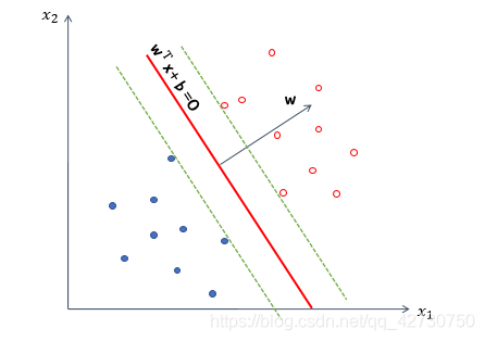
  The core idea of ​​the support vector machine classification method is to find a hyperplane in the feature space as the decision boundary to divide the samples into positive and negative classes, and make the generalization error of the model on the unknown data set as small as possible.

  Hyperplane: In geometry, a hyperplane is a subspace of a space, which is a space whose dimension is one less than the space in which it resides. If the data space itself is three-dimensional, its hyperplane is a two-dimensional plane, and if the data space itself is two-dimensional, its hyperplane is a one-dimensional line.

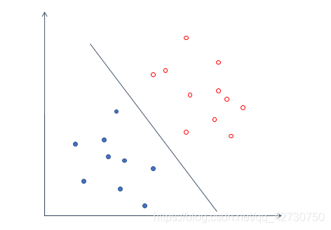
  For example, the above set of data, we can easily draw a line to divide the above data into two categories, and the error is zero. For a data set, there may be many hyperplanes with an error of 0, such as the following:

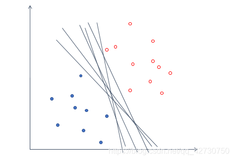
  But such a model cannot guarantee good generalization performance, that is, it cannot guarantee that this hyperplane also performs well on unknown data sets. So we introduce a noun ------ 间隔$\left(margin\right)$ is to translate the hyperplane we found to both sides until it stops at the sample point closest to the hyperplane to form two new hyperplanes. The distance between the two hyperplanes is It is called "interval", and the hyperplane is in the middle of this "interval", that is, the distance between the hyperplane we choose and the two new hyperplanes after translation is equal. The few sample points closest to the hyperplane are called支持向量$(support$ $vector)$。

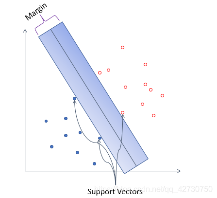
  Comparing the above two figures, intuitively, the samples can be divided into two categories, but if some noise is added to it, it is obvious that the blue hyperplane has the best tolerance to local disturbances, because It's "wide enough", if you can't imagine it, look at the following example:

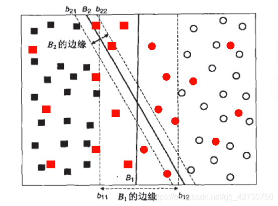
  Obviously, after introducing some new data samples, $B_1$This hyperplane error is still 0, and the classification result is the most robust, $B_2$This hyperplane has a classification error because of the small interval. Therefore, when we are looking for a hyperplane, we hope that the larger the interval, the better.
  The above is the support vector machine, that is, 通过找出间隔最大的超平面，来对数据进行分类the classifier of .
  The model of support vector machine can be divided into the following three types from simple to complex:
  $\bullet$ Linearly Separable Support Vector Machines
  $\bullet$ Linear Support Vector Machines
  $\bullet$ Nonlinear SVM
  Maximization via hard margin$(hard$ $margin$ $maxximization)$ , learn a linear classifier, that is, linearly separable support vector machine, also known as hard margin support vector machine; when the training data set is approximately linearly separable, maximize the$(soft$ $margin$ $maxximization)$ , also learn a linear classifier, that is, linear support vector machine, also known as soft margin support vector machine; when the training data set is linearly inseparable, by using the kernel technique (kernel ($(kernel$ $trckk)and$ soft margin maximization, learning nonlinear support vector machines.

  Simplicity is the foundation of complexity, and it is also a special case of complexity.

2. Function equation description

D = { ( x 1 , y 1 ) , ( x 2 , y 2 ) , … , ( xn , yn ) } , yi ∈ { − 1 , + 1 } D=\{(x_1,y_1   ) ),(x_2,y_2),\dots,(x_n,y_n)\},y_i \in \{-1,+1\}D={(x1​,y1​),(x2​,y2​),…,(xn​,yn​)},yi​∈{ −1,+ 1 } , in the above sample space, any line can be expressed as:$${\mathbf{w}}^T\mathbf{x}+b=0$$  其中$w=(w_1,w_2,\dots ,w_d{)}^T$ is the normal vector, which determines the direction of the hyperplane;$b$ is the displacement term, which determines the distance between the hyperplane and the origin. Obviously, the hyperplane can also be normal vector$w$ and displacement$bOK$ .
  For the convenience of derivation and calculation, we make the following regulations:
  points above the hyperplane are marked as positive, and points below the hyperplane are marked as negative, that is, for$(x_i,y_i)\in D$，若$y_i=+1$，则有${\mathbf{w}}^T{\mathbf{x}}_i+b>0$；若$y_i=-1$，则有$w^T{x}_i+b<0$，表达式如下：$$\{\begin{array}{ll}{w}^T{x}_i+b\ge +1,& y_i=+1\\ & \\ w^T{x}_i+b\le -1,& y_i=-1\end{array}$$  Among them, +1和-1表示两条平行于超平面的虚线到超平面的相对距离.
  Then, any point $The\; distance\; from\; x$ to the hyperplane can be written as:$$r=\frac{|{\mathbf{w}}^T+b|}{||\mathbf{w}||}$$  From this, the sum of the distances from the support vectors of two different labels to the hyperplane, that is, the interval, can be expressed as: $$c=\frac{2}{||w||}$$  Our goal is to find the hyperplane with the largest interval, that is, the parameter $w$ and$b$ , such that$\gamma$最大，即$$\begin{gathered} \underset{\mathbf{w},b}{\max }\frac{2}{||w||} \\ subjectto{y}_i({\mathbf{w}}^T{\mathbf{x}}_i+b)\ge 1,i=1,2,\dots ,n \end{gathered}$$   Obviously, maximizing the interval$\gamma$ only needs to be minimized$||w||$ is enough, so the constraints become as follows:$$\begin{gathered} \underset{\mathbf{w},b}{\min }\frac{1}{2}||\mathbf{w}|{|}^2 \\ subjectto{y}_i({\mathbf{w}}^T{x}_i+b)\ge 1,i=1,2,\dots ,n \end{gathered}$$

  In fact, it is to take the reciprocal, so why add the square, as I said before, $L_2$Paradigm Well, adding a square is to eliminate the operation of square root and simplify the calculation process.

3. Parameter solution

  To solve optimization problems with constraints, it is commonly used to introduce the Lagrange multiplier $\lambda$ constructs the Lagrangian function. In fact, this belongs to the conditional extremum problem of multivariate functions. You can refer to the conditional extremum of multivariate functions and the Lagrange multiplier method (standard\ Lagrange\ multiplier\ method)in the second volume of high mathematics.$\left(standdardLagrangemultipliermethod\right)$ , let's briefly review it below.

3.1 Lagrangian multipliers

  To find the function $z=f(x,y)$ in the additional condition$\phi (x,y)=$For the possible extreme points under$0$$$L(x,y)=f(x,y)+\lambda \phi (x,y)$$   where,$\lambda$ is a parameter, find its pair$x$、$y$和λ \lambdaThe first partial derivative of$\lambda$$$\{\begin{array}{l}{f}_x(x,y)+l{f}_x(x,y)=0\\ \\ f_y(x,y)+l{f}_y(x,y)=0\\ \\ \phi (x,y)=0\end{array}$$  With this system of equations solve $x$、$y$和$\lambda$ , the obtained$(x,y)$ is the function$f(x,y)$ in the additional condition$\phi (x,y)=$Possible extreme points below$0\; .$
  If the function has more than two independent variables and more than one additional condition, for example, the function$$u=f(x,y,z,t)$$ under the additional condition$$\begin{gathered} \phi (x,y,z,t)=0 \\ \psi (x,y,z,t)=0 \end{gathered}$$ , you can first make the Lagrangian function$$L(x,y,z,t)=f(x,y,z,t)+\lambda f(x,y,z,t)+\mu f(x,y,z,t)$$   among them,$l,\mu$ is a parameter, find its pair$x$、$y$、$z$、$t$、$\lambda$和$\mu$ 's first-order partial derivative, and make it zero, then solve the simultaneous equations to get$(x,y,z,t)$。

  Come, let's look at a small problem:
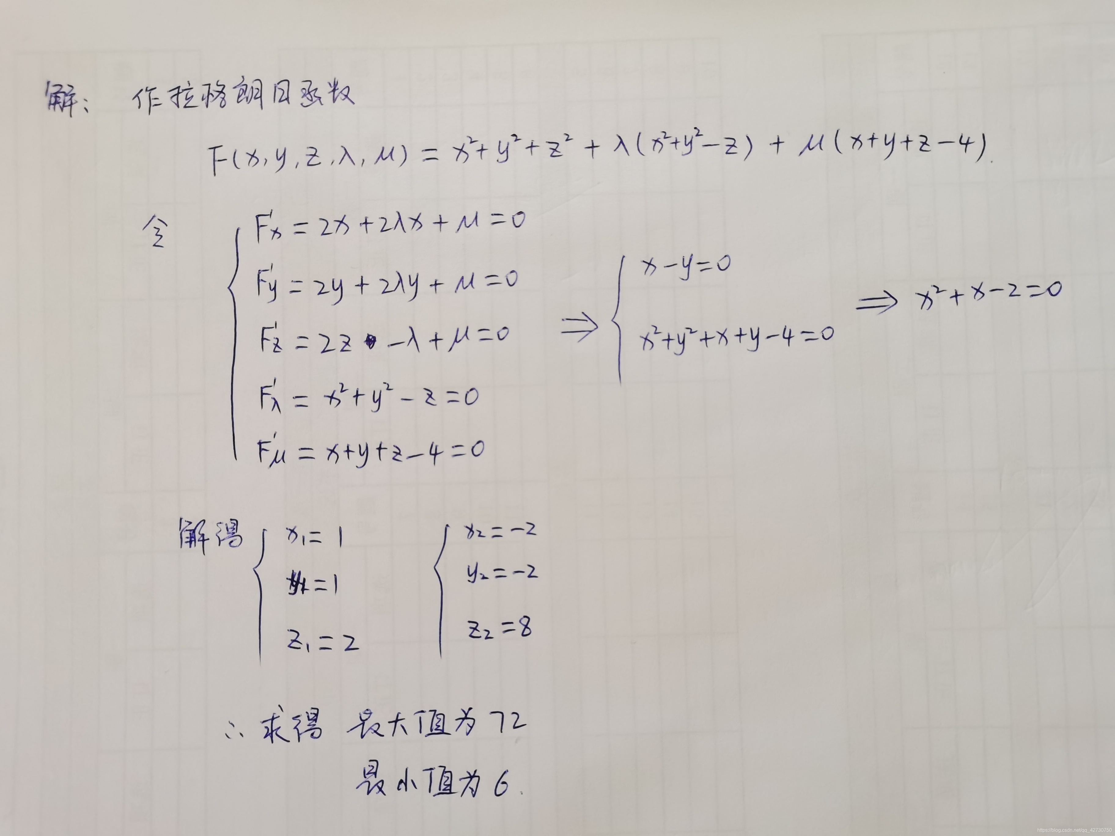
  find the function $u=x^2+y^2+z^2$ in the constraints$z=x^2+y^2$和$x+y+z=$The maximum and minimum values ​​under$4\; .$

3.2 Lagrangian dual function

  Convex optimization problems: the function itself is quadratic $\left(quadratic\right)$ , the constraints of the function are linear under its parameters, such a function is called a convex optimization$problem$$.$

  First construct the Lagrange function of the support vector machine, that is, the loss function: $$L(\mathbf{w},b,a)=\frac{1}{2}||\mathbf{w}|{|}^2+\sum _{i=1}^m{a}_i(1-y_i({\mathbf{w}}^T{\mathbf{x}}_i+b)\left)\right(a{}_i\ge 0)$$   among them，$a=(a_1,a_2,\dots ,a_n{)}^{T.}$ _
  It can be seen that the Lagrange function is divided into two parts: the first part is the same as our original loss function, and the second part expresses our constraints. We hope that the constructed loss function can not only represent our original loss function and constraints, but also express that we want to minimize the loss function to solve$w$ and$The\; intention\; of\; b$ , so we have to start with$\alpha$ is a parameter, solve$L(\mathbf{w},b,\alpha )$ , then$w$ and$b$ is a parameter, solve$L(\mathbf{w},b,\alpha )$ minimum value. Therefore, our goal can be written as follows:$$\underset{\mathbf{w},b}{\min }\underset{a_i\ge 0}{\max }L(w,b,a)(a{}_i\ge 0)$$