[CNN Basics] This article explains in detail how backpropagation (Backpropagation) is implemented in CNN - convolution and pooling (Part 1)

written in front

Inspired by the big homework of the course, I carefully studied the specific implementation process of backpropagation.
Thanks to the great gods from all walks of life for the articles written in related aspects.
We all know that CNN has both forward propagation and backpropagation during training, but only one line of code is needed to implement backpropagation in Pytorch. We don't have to implement them manually. Therefore, most deep learning books don't cover it either. The article will analyze
from three parts : convolutional layer, pooling layer, and batch normalization .

text

1. Backpropagation in convolutional layers

Refer to Pavithra Solai 's blog.

1.1 The chain rule

Before starting the formula derivation, we must first understand the calculation of the chain rule.
This part is relatively basic, if you know it in advance, you can skip it directly.
Let's give two examples to illustrate:

Case1

Take y=g(x), z=h(y).

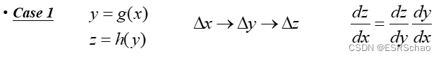
When x is changed, x affects y through g, and when y is changed, y affects z through h.
So if we want to calculate dz/dx, we can calculate dz/dy times dy/dx due to this effect.

Case2

Take x=g(s), y=g(s).

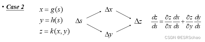
Then there is a function k that takes x and y to get z. Therefore, a change to s affects both x and y, causing x and y to affect z at the same time. Then when we calculate dz/ds. What we need to calculate is $\frac{\partial z}{\partial x}\frac{dx}{ds}+\frac{\partial z}{\partial y}\frac{dy}{ds}$。

This is the chain rule.

Now we propose a simple computational graph

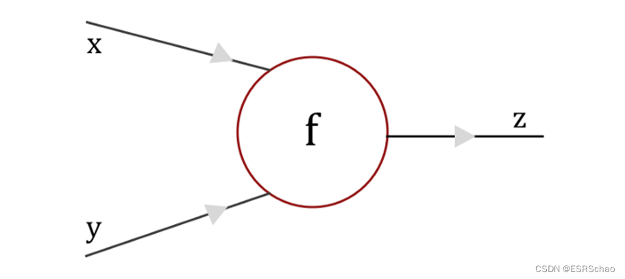
We can imagine a CNN as this simplified computational graph. Suppose we have a gate f in this computational graph that takes input x and y and outputs z.
We can easily compute the local gradient - differentiating z with respect to x and y is $\partial z/\partial x$和$\partial z/\partial y$。

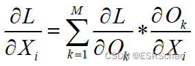
For the forward propagation of the convolutional layer, the input X and F pass through the convolutional layer, and finally use the loss function to obtain the loss L. When we start to calculate the loss in reverse, between layers, we get the gradient of the loss from the previous layer, ie $\partial L/\partial X$和$\partial L/\partial F$。

1.2 Forward Propagation

We start with the forward pass, using 3×3 inputs $X$ and 2×2 convolution kernel$F$ is convolved to get a 2×2 result$O$ , as shown in the figure below:

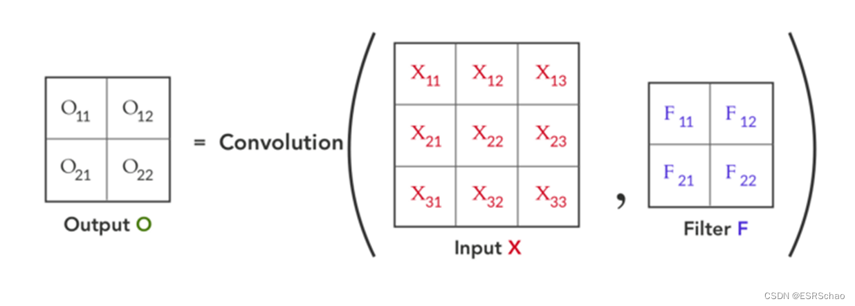
the process of convolution can be visualized as follows:

based on the forward propagation formula, we can perform backpropagation calculations.
As shown above, we can find relative to the outputOOThe local gradient of$O$$\partial O/\partial X$ and$\partial O/\partial F$ . Use the loss gradient of the previous layer -$\partial L/\partial O$ , and using the chain rule, we can calculate$\partial L/\partial X$ and$\partial L/\partial F$ up.

PS: Why do we need to calculate $\partial L/\partial X$ and$\partial L/\partial F$？

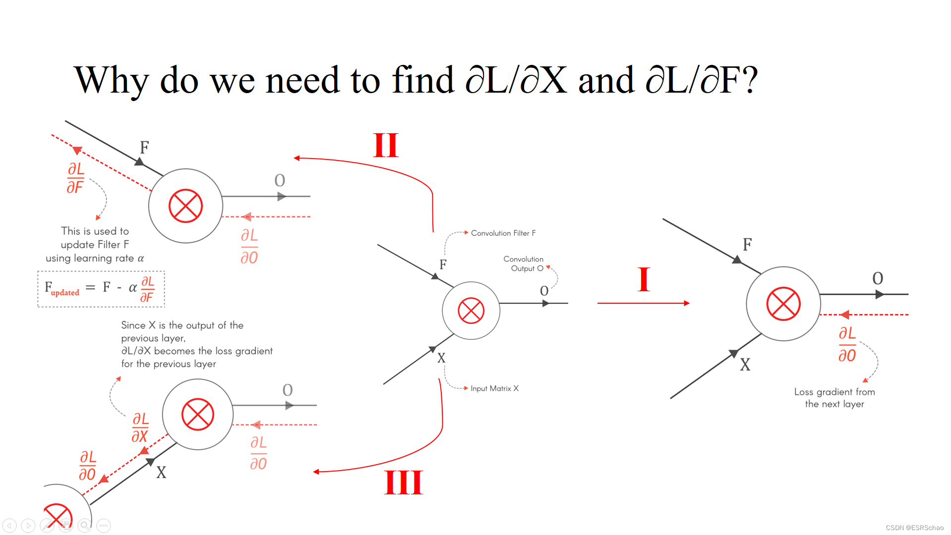
(1) 根据公式$F_{updated}=F-a\frac{\partial L}{\partial F}$It can be seen that $F$ is the parameter we need to calculate the update, and its update is through$\partial L/\partial F$ parameters to achieve.
(2)$\partial L/\partial X$ is used as the input part of this layer, which can be regarded as the output of back propagation during backpropagation, and this output is the input gradient of the previous layer, with$\partial L/\partial X$ we can continue the backpropagation calculation of the previous layer.

1.3 ∂O/∂F

The first step is the local gradient ∂O / ∂F ∂O/∂FCalculation of$\partial$$O$$/$$\partial$$F$

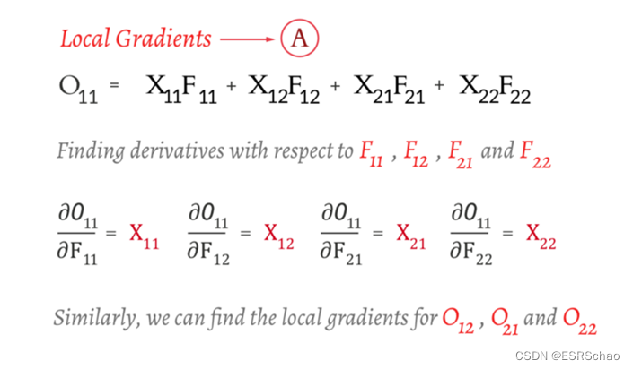
O $O_{11}$For example, we only need $O_{11}$The corresponding FF in the formulaIt is enough to find the partial derivative of$F.$This step is easy.

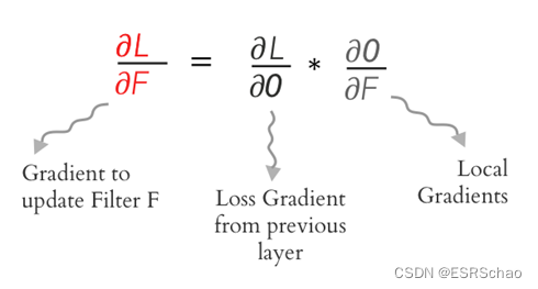
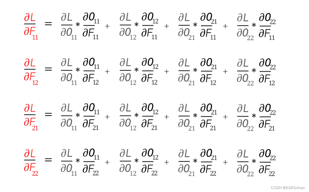
Then using the chain rule we can get $\partial L/\partial F$ , available via$\partial L/\partial O$ and$\partial O$ / ∂F ∂O/$\partial F$$The\; convolution\; of\; \partial O/\partial F$ is obtained. We use the following formula to expand it:

the expansion can lead to the following four formulas:

according to the partial derivative mentioned before, we can get:

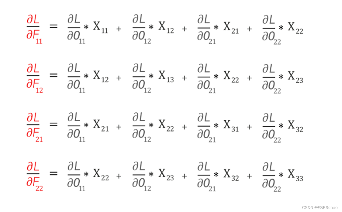
it can be expressed as input$X$ and loss gradient∂L/∂O ∂L/∂OThe convolution operation between$\partial$$L$$/$$\partial$$O\; is\; shown\; below.$

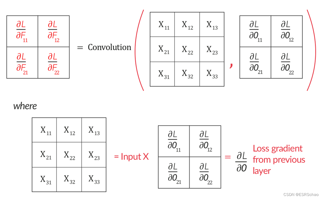
Thus we find$\partial O/\partial F$ , followed by$\partial O/\partial X$。

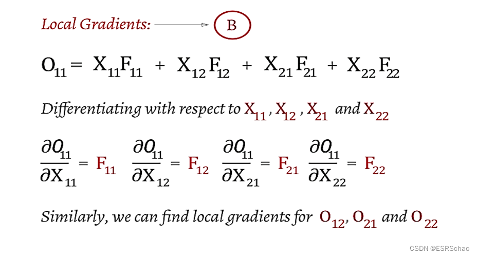
1.4 ∂O/∂X

and before solving for $The\; process\; of\; \partial O/\partial F$ is similar, or$O_{11}$For example, this time we need to $O_{11}$The corresponding $X$ seeks the partial derivative.

In this way, we get a new gradient. Using the chain rule, we can write a new convolution:

expand and calculate the partial derivative to get:

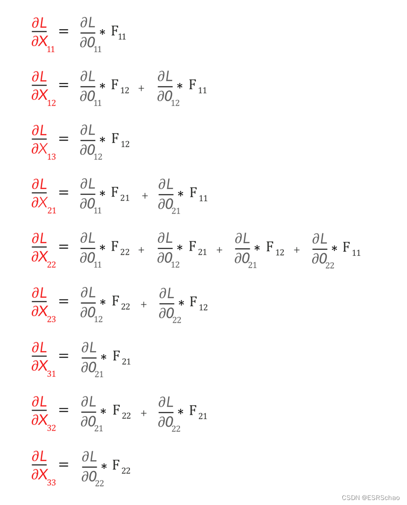
these 9 formulas are irregular at first glance, but they still conform to the calculation rules of convolution.
What are the specific rules? Let's first set$F$ rotates 180 degrees, which can be done by first flipping vertically and then horizontally.

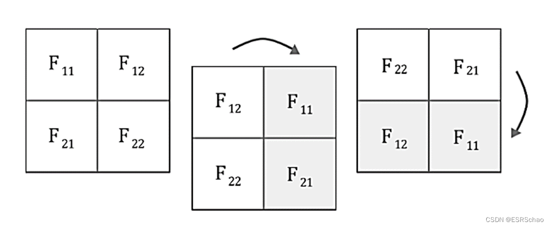
Then we perform a full mode convolution operation on it (for explanations of several modes of convolution, please refer to this blogger's blog post).
'Full-Convolution' can be visualized as shown below:

The above convolution operation generates $\partial L/\partial X$ , so we can put$\partial L/\partial X$ is expressed as follows:

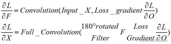
Now we have found $\partial L/\partial X$ and$\partial L/\partial F$ , we can now draw this conclusion:
the forward pass and back pass of the convolutional layer are both convolutions.
The conclusion can be expressed by the following formula.

2. Backpropagation in the pooling layer

This part refers to the blog post of Mr. Lei Mao .

Since the pooling layer does not have any learnable parameters, backpropagation is just an upsampling operation of the upstream derivative.
Here we take Max Pooling as an example for analysis.

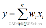
in: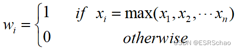

It can be seen from the formula of Max Pooling that when $When\; x$ is the maximum value, the weight wwobtained after partial derivative of the input and output$w$ will take 1. Right now:

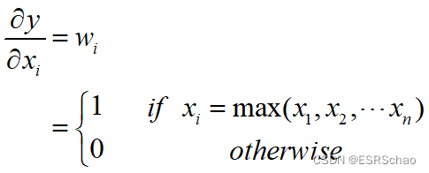
According to this formula, we can conclude that
the backpropagation of Max Pooling has no gradient for non-maximum values.

Due to space reasons, the Batch Normalization part will be explained in the second half.