Table of contents
1) Two-dimensional acoustic wave equation:
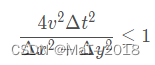
2) Convergence conditions (not very clear)
4) Two-dimensional space attenuation function
5) Boundary absorption conditions (not very clear..)
2) Reker wavelet and two-dimensional space attenuation function
3) Boundary absorption condition
4) Wave equation, iterative formula:
5) The whole code is as follows:
3. Realization of two-dimensional wave equation based on matlab
Numerical solution of wave equation is one of the core technologies of wave equation forward modeling, reverse time migration and full waveform inversion. In this paper, the second-order finite difference is used to discretize the wave equation, and then the numerical solution of the wave equation is realized, and its propagation process in the medium is simulated.
NumPy is usually used together with SciPy (Scientific Python) and Matplotlib (drawing library). This combination is widely used to replace MatLab. It is a powerful scientific computing environment that helps us learn data science or machine learning through Python.
SciPy includes modules for optimization, linear algebra, integration, interpolation, special functions, fast Fourier transforms, signal and image processing, ordinary differential equation solving, and other calculations commonly used in science and engineering.
Matplotlib is a visual interface for the Python programming language and its numerical mathematics extension package NumPy. It provides an application programming interface (API) for drawing embedded in applications using common GUI toolkits such as Tkinter, wxPython, Qt or GTK+.
The code part of this article only uses the NumPy and Matplotlib packages.
1. Principle:
1) Two-dimensional acoustic wave equation:

Where u is the sound pressure, f is the sound pressure at the source center, x/z is the sampling point in the x/z direction, t is the time, and v is the velocity.
Using Taylor's formula to expand:
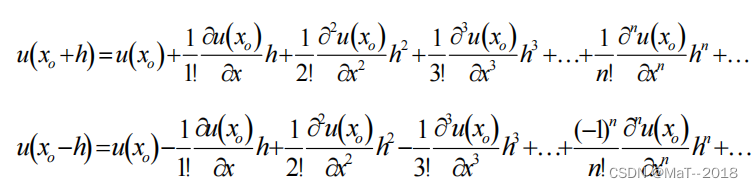
Adding the two formulas gives:
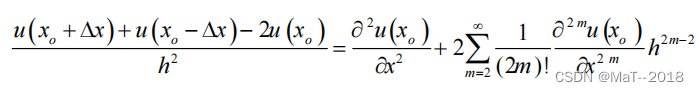
Then there are:

Approximate second-order difference operator :
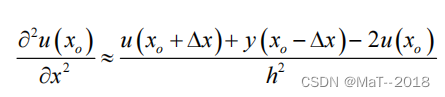
Discretize the second derivative using the second central difference operator:
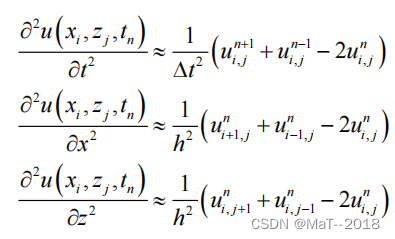
Substitute the above formula into the acoustic wave equation to get the second-order central difference scheme:
![]()
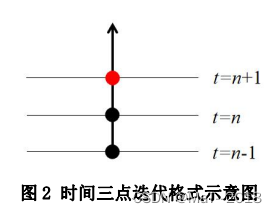
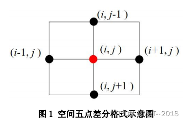
The schematic diagram of its space and time difference format is shown in the figure below:
2) Convergence conditions (not very clear)
3) Lake wavelet
The Lake wavelet is one of the seismic wavelets. The seismic wave excited by the seismic source, propagated underground and received by people on the ground or in the well is usually a short pulse vibration, which is called a vibration wavelet, as shown in the figure below.
The formula is: f(t)=(1-2*(pi*f*t)^2)*exp(-(pi*f*t)^2), where t is the time and f is the main frequency.
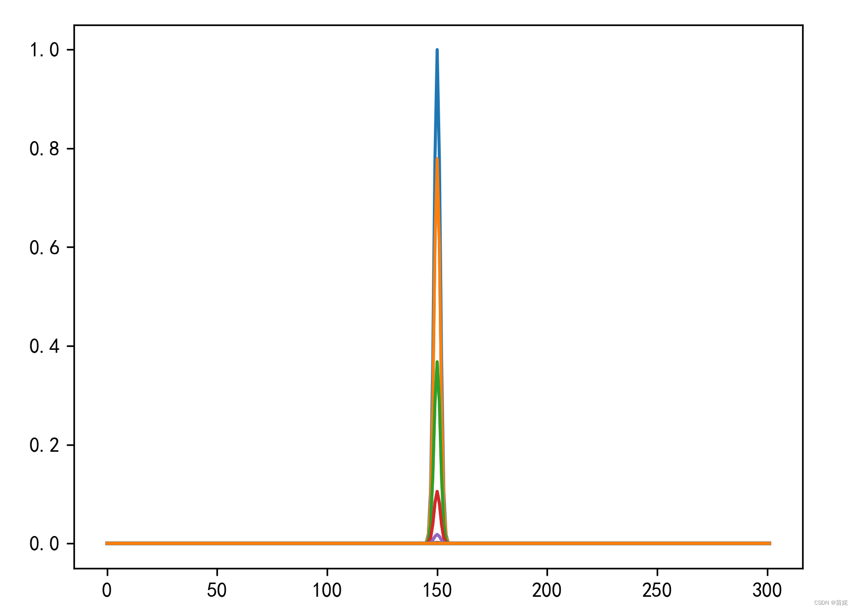
4) Two-dimensional space attenuation function
The source center is 1, no attenuation, the farther away from the center, the greater the attenuation.
h_x_z =  np.zeros((Nx+1,Nz+1))  #np.exp(-0.25 * ((x - Nx//2)**2 + (z - Nz//2)**2))  二维空间衰减函数
h_x_z[Nx//2,Nz//2] = 1   # 在Nx//2,Nz//2处激发
h_x_z =  np.exp(-alpha ** 2 * ((x - Nx//2)**2 + (z - Nz//2)**2))  # 二维空间衰减函数
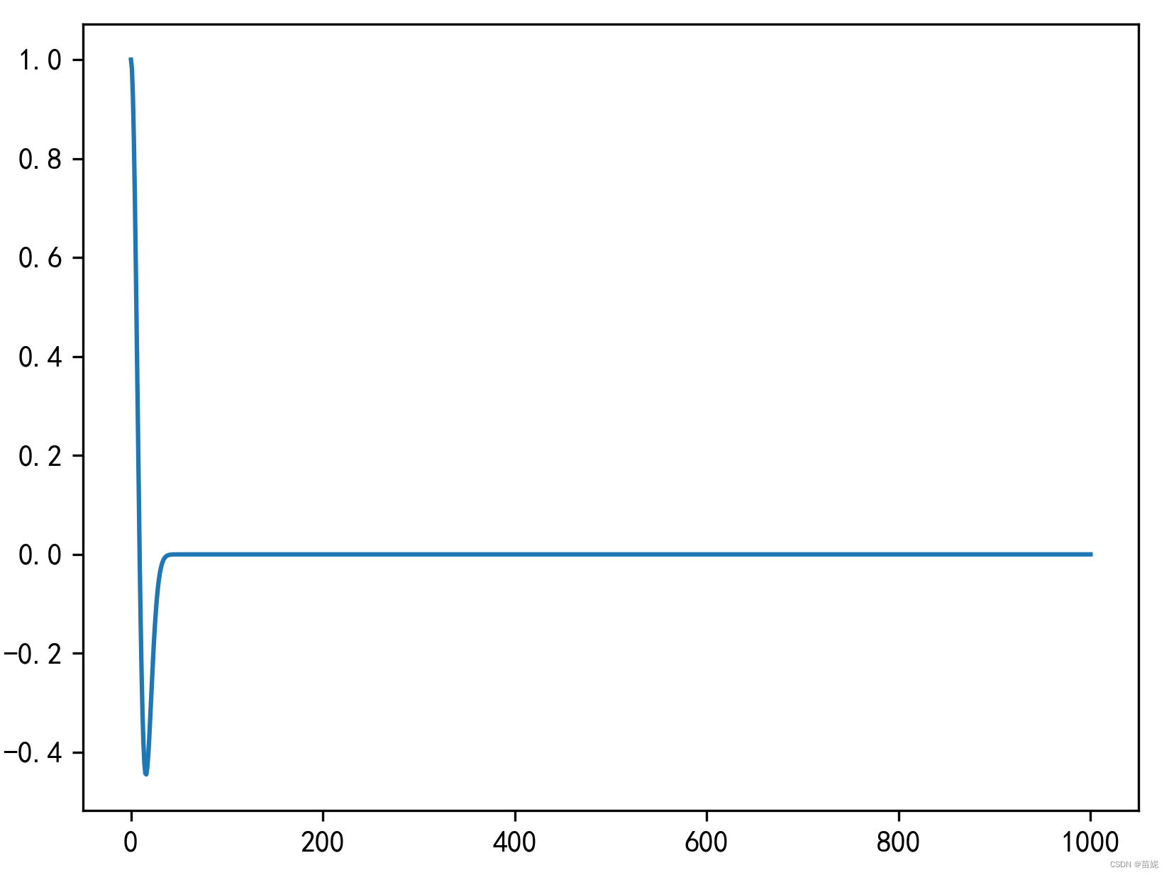
The figure below shows the curve of h_x_z[150], the entire two-dimensional space attenuation coefficient h_x_z, with [150,150] as the center (shock source), attenuates around.
5) Boundary absorption conditions (not very clear..)
Function: There is no boundary when the sound wave propagates, so there is no boundary reflection problem. However, due to the limited observation range during forward simulation, there must be a boundary. The boundary absorption condition is to absorb energy as much as possible and minimize boundary reflection. (My understanding, welcome to discuss) The following are two boundary absorption conditions. The PML condition is more commonly used now.
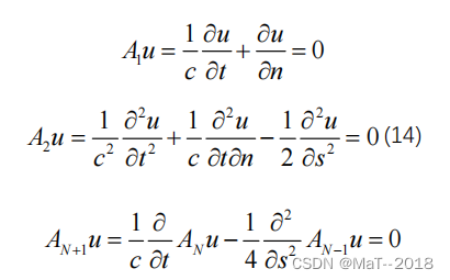
Clayton-Engquist mono-wave absorbing boundary condition: It was first discovered and promoted by Clayton et al., and its differential expression is:
Among them: n is the outer normal direction of the boundary; s is the tangent direction of the boundary.
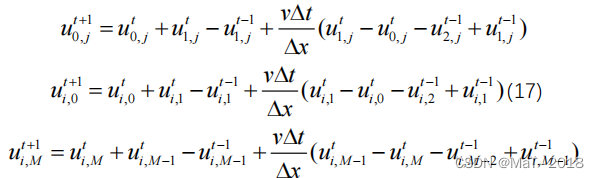
Discretize the above formula to get the upper, lower, left, and right boundary difference format as follows:
where:N and M are the grid numbers of the boundary.


Reynolds boundary conditions: For the two-dimensional acoustic wave equation, the differential operator of the two-dimensional acoustic wave equation can be used to obtain:
By discretizing the above formula, the calculation formula of the upper, lower, left, and right boundaries can be obtained:

2. Programming implementation
1) Parameter setting:
- The length in the x/z direction is 1500m, the space step in the x/z direction is 5m, and the number of sampling points in each direction is 301;
- The simulation time is 1s, the time step is 0.001s, and the number of time samples is 1000;
- The source frequency is 25Hz;
- Space attenuation factor 0.5;
- The wave speed is fixed, 3000m/s at any position
- The source location is at the center; the initial sound pressure is zero.
# 区域大小
Nx = 301
Nz = 301
# 空间间隔
dx = h
dy = h

# 时间采样数
Nt = 1000
# 时间步
dt = 1 / Nt

# 速度模型
v = np.ones((Nx+1,Nz+1)) * 3000
u = np.zeros((Nt+1,Nx+1,Nz+1))
h = 5

# 子波主频
fm = 25
# 空间衰减因子
alpha = 0.5

# 迭代公式中的r
A = v **2 * dt ** 2 / h ** 2
C = v * dt / h
2) Reker wavelet and two-dimensional space attenuation function
t = np.arange(0, Nt+1)
t0 = 0  # 延迟时间,相当于在t=t0时激发 ,震幅在t0时最大,相位也在此
s_t = (1 - 2 * (np.pi * fm * dt * (t - t0)) ** 2) * np.exp( - (np.pi * fm * dt * (t - t0)) ** 2)

x = np.arange(0,Nx+1)
z = np.arange(0,Nz+1)
x,z = np.meshgrid(x,z)

h_x_z =  np.zeros((Nx+1,Nz+1))  #np.exp(-0.25 * ((x - Nx//2)**2 + (z - Nz//2)**2))  二维空间衰减函数
h_x_z[Nx//2,Nz//2] = 1   # 在Nx//2,Nz//2处激发
h_x_z =  np.exp(-alpha ** 2 * ((x - Nx//2)**2 + (z - Nz//2)**2))  # 二维空间衰减函数

x0 = Nx // 2
z0 = Nz // 2
u0 = lambda r, s: 0.25*np.exp(-((r-x0)**2+(s-z0)**2))
JJ = np.arange(1,Nz)
II = np.arange(1,Nx)
II,JJ = np.meshgrid(II,JJ)
3) Boundary absorption condition
# 边界条件
ii = np.arange(Nx+1)
jj = np.arange(Nz+1)
# Clayton-Engquist-majda 二阶吸收边界条件
u[t+1,  0, jj] = (2 - 2 * C[ 0, jj] - C[ 0, jj] ** 2) * u[t,  0, jj] \
                        + 2 * C[ 1, jj] * (1 + C[ 1, jj]) * u[t,  1, jj] \
                        - C[ 2, jj] ** 2 * u[t,  2, jj] \
                        + (2 * C[ 0, jj] - 1) * u[t - 1,  0, jj] \
                        - 2 * C[ 1, jj] * u[t - 1,  1, jj]


# 下部
u[t+1, -1, jj] = (2 - 2 * C[ -1, jj] - C[ -1, jj] ** 2) * u[t,  -1, jj] \
                        + 2 * C[ -2, jj] * (1 + C[ -2, jj]) * u[t,  -2, jj] \
                        - C[ -3, jj] ** 2 * u[t,  -3, jj] \
                        + (2 * C[ -1, jj] - 1) * u[t - 1,  -1, jj] \
                        - 2 * C[ -2, jj] * u[t - 1,  -2, jj]

# 左部
u[t+1, ii,  0] = (2 - 2 * C[ii,  0] - C[ii,  0] ** 2) * u[t,  ii, 0] \
                        + 2 * C[ii,  1] * (1 + C[ii,  1]) * u[t,  ii, 1] \
                        - C[ii,  2] ** 2 * u[t,  ii, 2] \
                        + (2 * C[ii,  0] - 1) * u[t - 1,  ii, 0] \
                        - 2 * C[ii,  1] * u[t - 1,  ii, 1]
# 右部
u[t+1, ii, -1] = (2 - 2 * C[ii,  -1] - C[ii,  -1] ** 2) * u[t,  ii, -1] \
                        + 2 * C[ii,  -2] * (1 + C[ii,  -2]) * u[t,  ii, -2] \
                        - C[ii,  -3] ** 2 * u[t,  ii, -3] \
                        + (2 * C[ii,  -1] - 1) * u[t - 1,  ii, -1] \
                        - 2 * C[ii,  -2] * u[t - 1,  ii, -2]
#Reynolds 边界条件
u[t+1,ii, 0] = u[t,ii, 0] + u[t,ii, 1] - u[t-1,ii, 1] + C[ii, 1]*u[t,ii, 1] - C[ii, 0]*u[t,ii, 0] -C[ii, 2]*u[t-1,ii, 2] +C[ii, 1]*u[t-1,ii, 1]

u[t+1,ii,-1] = u[t,ii,-1] + u[t,ii,-2] - u[t-1,ii,-2] + C[ii,-2]*u[t,ii,-2] - C[ii,-1]*u[t,ii,-1] -C[ii,-3]*u[t-1,ii,-3] +C[ii,-2]*u[t-1,ii,-2]

u[t+1, 0,jj] = u[t, 0,jj] + u[t, 1,jj] - u[t-1, 1,jj] + C[ 1,jj]*u[t, 1,jj] - C[ 0,jj]*u[t, 0,jj] -C[ 2,jj]*u[t-1, 2,jj] +C[ 1,jj]*u[t-1, 1,jj]

u[t+1,-1,jj] = u[t,-1,jj] + u[t,-2,jj] - u[t-1,-2,jj] + C[-2,jj]*u[t,-2,jj] - C[-1,jj]*u[t,-1,jj] -C[-3,jj]*u[t-1,-3,jj] +C[-1,jj]*u[t-1,-2,jj]
4) Wave equation, iterative formula:
# 迭代公式
u[t+1,II,JJ] = s_t[t]*h_x_z[II,JJ]+A[II,JJ]*(u[t,II,JJ+1]+u[t,II,JJ-1]+u[t,II+1,JJ]+u[t,II-1,JJ])+(2-4*A[II,JJ])*u[t,II,JJ]-u[t-1,II,JJ]
5) The whole code is as follows:
import numpy as np
import imageio
import os
import pandas as pd
from matplotlib import pyplot as plt
# 解决中文问题
plt.rcParams['font.sans-serif'] = ['SimHei']
# 解决负号显示问题
plt.rcParams['axes.unicode_minus'] = False


Nx = 301
Nz = 301
Nt = 1000
v = np.ones((Nx+1,Nz+1)) * 3000
h = 5
fm = 25
alpha = 0.5
dt = 1 / Nt
dx = h
dy = h
A = v **2 * dt ** 2 / h ** 2
C = v * dt / h

r = np.max(v)*dt/h
assert r < 0.707,f'r should < 0.707, but is {r}'
u = np.zeros((Nt+1,Nx+1,Nz+1))


t = np.arange(0, Nt+1)
t0 = 0  # 延迟时间,相当于在t=t0时激发 ,震幅在t0时最大,相位也在此
s_t = (1 - 2 * (np.pi * fm * dt * (t - t0)) ** 2) * np.exp( - (np.pi * fm * dt * (t - t0)) ** 2)

plt.plot(s_t)
plt.show()

x = np.arange(0,Nx+1)
z = np.arange(0,Nz+1)
x,z = np.meshgrid(x,z)
# print(((z - Nz//2)**2).shape)


h_x_z =  np.zeros((Nx+1,Nz+1))  #np.exp(-0.25 * ((x - Nx//2)**2 + (z - Nz//2)**2))  二维空间衰减函数
h_x_z[Nx//2,Nz//2] = 1   # 在Nx//2,Nz//2处激发
h_x_z =  np.exp(-alpha ** 2 * ((x - Nx//2)**2 + (z - Nz//2)**2))  # 二维空间衰减函数


JJ = np.arange(1,Nz)
II = np.arange(1,Nx)
II,JJ = np.meshgrid(II,JJ)

mode = 'c_e'
img_path = './2_order'
if not os.path.exists(img_path):
    os.makedirs(img_path)

for t in range(2,Nt):
    print('\rstep {} / {}'.format(t ,Nt), end="")

    # 边界条件
    ii = np.arange(Nx+1)
    jj = np.arange(Nz+1)
    if mode == 'c_e':
        # Clayton-Engquist-majda 二阶吸收边界条件
        u[t+1,  0, jj] = (2 - 2 * C[ 0, jj] - C[ 0, jj] ** 2) * u[t,  0, jj] \
                                + 2 * C[ 1, jj] * (1 + C[ 1, jj]) * u[t,  1, jj] \
                                - C[ 2, jj] ** 2 * u[t,  2, jj] \
                                + (2 * C[ 0, jj] - 1) * u[t - 1,  0, jj] \
                                - 2 * C[ 1, jj] * u[t - 1,  1, jj]


        # 下部
        u[t+1, -1, jj] = (2 - 2 * C[ -1, jj] - C[ -1, jj] ** 2) * u[t,  -1, jj] \
                                + 2 * C[ -2, jj] * (1 + C[ -2, jj]) * u[t,  -2, jj] \
                                - C[ -3, jj] ** 2 * u[t,  -3, jj] \
                                + (2 * C[ -1, jj] - 1) * u[t - 1,  -1, jj] \
                                - 2 * C[ -2, jj] * u[t - 1,  -2, jj]

        # 左部
        u[t+1, ii,  0] = (2 - 2 * C[ii,  0] - C[ii,  0] ** 2) * u[t,  ii, 0] \
                                + 2 * C[ii,  1] * (1 + C[ii,  1]) * u[t,  ii, 1] \
                                - C[ii,  2] ** 2 * u[t,  ii, 2] \
                                + (2 * C[ii,  0] - 1) * u[t - 1,  ii, 0] \
                                - 2 * C[ii,  1] * u[t - 1,  ii, 1]
        # 右部
        u[t+1, ii, -1] = (2 - 2 * C[ii,  -1] - C[ii,  -1] ** 2) * u[t,  ii, -1] \
                                + 2 * C[ii,  -2] * (1 + C[ii,  -2]) * u[t,  ii, -2] \
                                - C[ii,  -3] ** 2 * u[t,  ii, -3] \
                                + (2 * C[ii,  -1] - 1) * u[t - 1,  ii, -1] \
                                - 2 * C[ii,  -2] * u[t - 1,  ii, -2]
    if mode == 're':
        #Reynolds 边界条件
        u[t+1,ii, 0] = u[t,ii, 0] + u[t,ii, 1] - u[t-1,ii, 1] + C[ii, 1]*u[t,ii, 1] - C[ii, 0]*u[t,ii, 0] -C[ii, 2]*u[t-1,ii, 2] +C[ii, 1]*u[t-1,ii, 1]

        u[t+1,ii,-1] = u[t,ii,-1] + u[t,ii,-2] - u[t-1,ii,-2] + C[ii,-2]*u[t,ii,-2] - C[ii,-1]*u[t,ii,-1] -C[ii,-3]*u[t-1,ii,-3] +C[ii,-2]*u[t-1,ii,-2]

        u[t+1, 0,jj] = u[t, 0,jj] + u[t, 1,jj] - u[t-1, 1,jj] + C[ 1,jj]*u[t, 1,jj] - C[ 0,jj]*u[t, 0,jj] -C[ 2,jj]*u[t-1, 2,jj] +C[ 1,jj]*u[t-1, 1,jj]

        u[t+1,-1,jj] = u[t,-1,jj] + u[t,-2,jj] - u[t-1,-2,jj] + C[-2,jj]*u[t,-2,jj] - C[-1,jj]*u[t,-1,jj] -C[-3,jj]*u[t-1,-3,jj] +C[-1,jj]*u[t-1,-2,jj]


    # 迭代公式
    u[t+1,II,JJ] = s_t[t]*h_x_z[II,JJ]*v[II, JJ]**2*dt**2+A[II,JJ]*(u[t,II,JJ+1]+u[t,II,JJ-1]+u[t,II+1,JJ]+u[t,II-1,JJ])+(2-4*A[II,JJ])*u[t,II,JJ]-u[t-1,II,JJ]


    plt.imshow(u[t], cmap='gray_r') # 'seismic' gray_r
    # plt.axis('off')  # 隐藏坐标轴
    plt.colorbar()
    if t % 10 == 0:
        plt.savefig(os.path.join(img_path, str(t) + '.png'),
                    bbox_inches="tight", # 去除坐标轴占用空间
                    pad_inches=0.0) # 去除所有白边
        plt.pause(0.05)

    plt.cla()
    plt.clf()  # 清除所有轴,但是窗口打开,这样它可以被重复使用
plt.close()

# 保存gif
filenames=[]
for files in os.listdir(img_path ):
    if files.endswith('jpg') or files.endswith('jpeg') or files.endswith('png'):
        file=os.path.join(img_path ,files)
        filenames.append(file)

images = []
for filename in filenames:
    images.append(imageio.imread(filename))

imageio.mimsave(os.path.join(img_path,  'wave.gif'), images,duration=0.0001)
reference:
3. Realization of two-dimensional wave equation based on matlab
close all
clear
clc

% 此程序是有限差分法实现声波方程数值模拟


%% 参数设置
delta_t = 0.001; % s
delta_s = 10; % 空间差分:delta_s = delta_x = delta_y (m)
nx = 800;
ny = 800;
nt = 1000;
fmain = 12.5;
%loop:按照10000s为一次大循环;slice代表每隔1000s做一个切片
loop_num = 3;
slice = 1000;
slice_index = 1;
%% 初始化
%震源
t = 1:nt;
t0 = 50;
s_t = (1-2*(pi*fmain*delta_t*(t-t0)).^2).*exp(-(pi*fmain*delta_t*(t-t0)).^2);%源
%一个loop代表向后计算10000s,目的是减少内存消耗
%间隔1000s保存一张切片
num_slice = nt*loop_num/slice;
U_loop(1:ny,1:nx,1:num_slice) = 0;
U_next_loop(1:ny,1:nx,1:2) = 0;
%初始化数组变量
w(1:ny,1:nx) = 0;
U(1:ny,1:nx,1:nt) = 0;
w(400,400) = 1;
V(1:ny,1:nx) = 2000;
A = V.^2*delta_t^2/delta_s^2;
B = V*delta_t/delta_s;

%% 开始计算
JJ = 2:ny-1;
II = 2:nx-1;
start_time = clock;
for loop = 1:loop_num
    fprintf('Loop=%d\n',loop)
    for i_t = 2:nt-1
        if(loop>1)
            s_t(i_t) = 0;
        end
        %上边界
        U(1,II,i_t+1) = (2-2*B(1,II)-A(1,II)).*U(1,II,i_t)+2*B(1,II).*(1+B(1,II)).*U(2,II,i_t)...
            -A(1,II).*U(3,II,i_t)+(2*B(1,II)-1).*U(1,II,i_t-1)-2*B(1,II).*U(2,II,i_t-1);
        %下边界
        U(ny,II,i_t+1) = (2-2*B(ny,II)-A(ny,II)).*U(ny,II,i_t)+2*B(ny,II).*(1+B(ny,II)).*U(ny-1,II,i_t)...
            -A(ny,II).*U(ny-2,II,i_t)+(2*B(ny,II)-1).*U(ny,II,i_t-1)-2*B(1,II).*U(ny-1,II,i_t-1);
        %左边界
        U(JJ,1,i_t+1) = (2-2*B(JJ,1)-A(JJ,1)).*U(JJ,1,i_t)+2*B(JJ,1).*(1+B(JJ,1)).*U(JJ,1+1,i_t)...
                            -A(JJ,1).*U(JJ,1+2,i_t)+(2*B(JJ,1)-1).*U(JJ,1,i_t-1)-2*B(JJ,1).*U(JJ,1+1,i_t-1);
        %右边界
        U(JJ,nx,i_t+1) = (2-2*B(JJ,nx)-A(JJ,nx)).*U(JJ,nx,i_t)+2*B(JJ,nx).*(1+B(JJ,nx)).*U(JJ,nx-1,i_t)...
                            -A(JJ,nx).*U(JJ,nx-2,i_t)+(2*B(JJ,nx)-1).*U(JJ,nx,i_t-1)-2*B(JJ,nx).*U(JJ,nx-1,i_t-1);
        %递推公式
        U(JJ,II,i_t+1) = s_t(i_t).*w(JJ,II)+A(JJ,II).*(U(JJ,II+1,i_t)+U(JJ,II-1,i_t)+U(JJ+1,II,i_t)+U(JJ-1,II,i_t))+...
                            (2-4*A(JJ,II)).*U(JJ,II,i_t)-U(JJ,II,i_t-1);
        if(mod(i_t,100)==0)
            run_time = etime(clock,start_time);
            fprintf('step=%d,total=%d,累计耗时%.2fs\n',i_t+(loop-1)*nt,nt*loop_num,run_time)
            U_loop(:,:,slice_index) = U(:,:,i_t);
            slice_index = slice_index +1;
        end
    end
    %处理四个角点
    KK = 1:nt;
    U(1,1,KK) = 1/2*(U(1,2,KK)+U(2,1,KK));
    U(1,nx,KK) = 1/2*(U(1,nx-1,KK)+U(2,nx,KK));
    U(ny,1,KK) = 1/2*(U(ny-1,1,KK)+U(ny,2,KK));
    U(ny,nx,KK) = 1/2*(U(ny-1,nx,KK)+U(ny,nx-1,KK));
    %% 为下一次loop做准备
    fprintf('step=%d,total=%d,累计耗时%.2fs\n',i_t+1+(loop-1)*nt,nt*loop_num,run_time)
    U_loop(:,:,slice_index) = U(:,:,nt);
    slice_index = slice_index +1;
    U_next_loop(:,:,1)=U(:,:,nt-1);
    U_next_loop(:,:,2)=U(:,:,nt);
    U(:,:,:) = 0;
    U(:,:,1) = U_next_loop(:,:,1);
    U(:,:,2) = U_next_loop(:,:,2);
end

%% 制作动图
fmat=moviein(num_slice);
filename = 'FDM_4_homogenerous.gif';
for II = 1:num_slice
    pcolor(U_loop(:,:,II));
    shading interp;
    axis tight;
    set(gca,'yDir','reverse');
    str_title = ['FDM-4-homogenerous  t=',num2str(delta_t*II*100),'s'];
    title(str_title)
    drawnow; %刷新屏幕
    F = getframe(gcf);%捕获图窗作为影片帧
    I = frame2im(F); %返回图像数据
    [I, map] = rgb2ind(I, 256); %将rgb转换成索引图像
    if II == 1
        imwrite(I,map, filename,'gif', 'Loopcount',inf,'DelayTime',0.1);
    else
        imwrite(I,map, filename,'gif','WriteMode','append','DelayTime',0.1);
    end
    fmat(:,II)=getframe;
end
movie(fmat,10,5);
%% 绘图为gif
pcolor(U_loop(:,:,num_slice))
shading interp;
axis tight;
set(gca,'yDir','reverse');
str_title = ['FDM-4-homogenerous  t=',num2str(delta_t*num_slice*100),'s'];
title(str_title)
colormap('Gray')
filename = [str_title,'.jpg'];
saveas(gcf,filename)

%% 耗时
toc