Data Analysis Training Chapter 8 Corporate Income Tax Forecast Analysis

Data Analysis Training Chapter 8 Corporate Income Tax Prediction Analysis (No Warning, No Error, Complete Analysis)

foreword

   These days, I took the time to revisit data mining. When I did this question again, I checked the answers on the Internet and found that many of them had some problems, so I wrote it myself. There is no error or warning in the code. You can use it with confidence.

1. Background introduction

1. Topic selection

Select the training task of Chapter 8 - Corporate Income Tax Forecasting and Analysis

2. Analyze the corporate income tax forecast background

(1) Introduction and requirements of corporate income tax

   Enterprise income tax is a kind of income tax levied on the production and operation income and other income of enterprises and other income-generating organizations in my country. In my country, the taxpayers of enterprise income tax are enterprises and other organizations that obtain income, including various enterprises, public institutions, social organizations, private non-enterprise units and other organizations engaged in business activities. The corporate income tax rate is a proportional tax rate of 25%, and 20% for non-resident enterprises. Enterprise income tax payable = taxable income of the current period * applicable tax rate, taxable income = total income - amount of allowed deductible items.

   my country's corporate income tax is only levied on profits, and a proportional tax rate is often used. Most enterprises bear the same tax burden level, which is conducive to promoting fairness. At the same time, the corporate income tax with a proportional tax rate is more conducive to promoting enterprises to improve their business management, strive to reduce costs, and increase profitability compared with progressive tax rates implemented in other countries. At the same time, my country's current corporate income tax is also conducive to the government's investment in taxpayers, industrial restructuring, and economic development. Corporate income tax is also one of the important ways to raise financial funds for national construction, which is of great significance.

   Prediction and analysis of corporate income tax is conducive to promoting the consciousness of corporate taxpayers to pay taxes consciously, is conducive to combating tax evasion, tax evasion and other behaviors, ensures the normal and stable progress of national taxation, and lays a solid financial foundation for national construction. Therefore, it is very necessary to establish a correct and effective enterprise income tax forecasting model.

(2) Basic situation of corporate income tax forecast data

   The data sets used in this modeling include the 2004–2015 total social fixed asset investment, urban commodity retail price index, total output value of the construction industry, retail sales of chain stores (companies) above designated size, etc.

(3) Objectives of corporate income tax forecast analysis

   a. Analyze and identify characteristic data that affect corporate income tax

   b. Establish a forecasting model to forecast corporate income tax in 2014 and 2015, and evaluate the model.

3. Understand corporate income tax forecasting methods

   By consulting textbooks, related papers and materials, it is found that using Lasso feature selection method to study the effect of corporate income tax is relatively better. This modeling is based on the Lasso feature selection, considering the excellent performance of gray prediction for a small amount of data prediction, a gray prediction model is established, and then the data results obtained by gray prediction are substituted into the trained model, so that the original data is fully considered. On the basis of this, a relatively accurate forecast result is obtained, that is, the corporate income tax in 2014 and 2015.

2. Training 1

1. Task description

   Carry out a correlation analysis on the original characteristics that affect corporate income tax, and interpret the correlation between the original characteristics and the correlation between the original characteristics and the target characteristics.

2. Task analysis

   The correlation function is used to calculate the correlation coefficient between the features, and the correlation analysis is carried out on the original data.

3. Training points

(1) Master the correlation analysis method in Python

  Correlation analysis refers to the analysis of two or more correlated feature elements to determine the degree of closeness of the two feature factors. The Pearson correlation coefficient is one of the simplest correlation coefficients, which can be used to judge the strength of the linear correlation between two features X and Y, usually expressed by r or ρ, and its value range is [-1,1].
The Pearson correlation coefficient is calculated as follows: If two vectors X=(x1,x2,…,xn), Y=(y1,y2,…yn), then the Pearson correlation
coefficient is:

(2) Understand and be able to use Python to realize the correlation analysis of the relevant characteristics of corporate income tax forecasting

(3) Interpretation of the correlation analysis results

4. Implementation ideas and steps

(1) Find the Pearson correlation coefficient between the original data features

(2) Judging the correlation between each feature

5. Task realization

Find the Pearson correlation coefficient between the original data features

import numpy as np
import pandas as pd
inputfile = '../data/income_tax.csv' #读取数据文件
data = pd.read_csv(inputfile) #读取数据
#保留两位小数
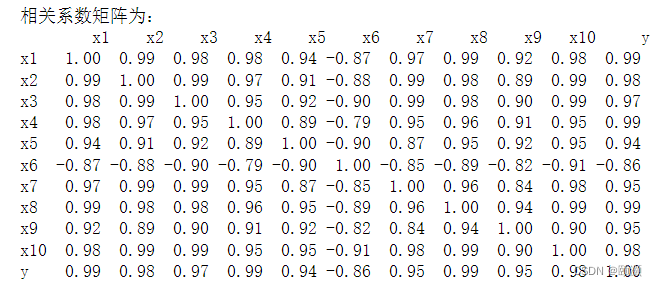
print('相关系数矩阵为：','\n',np.round(data.iloc[1:,1:].corr(method = 'pearson'), 2))

(2) Judging the correlation between each feature

   From the obtained Pearson correlation coefficient matrix, it can be seen that the correlation between the selected features and y is relatively strong, but the linear relationship between the loss surface (x6) and corporate income tax (y) of state-owned and state-holding industrial enterprises above a designated size shows a strong negative correlation. The rest of the features are all highly positively correlated with corporate income tax, in descending order of correlation, they are x1, x4, x8, x2, x10, X3, x7, x9, x5. At the same time, there is serious multicollinearity among the features, for example, features x2, x3, x10 have serious collinearity with features other than x6 and x9, x7, x8 and x1, x2 have serious collinearity,... …To sum up, the selected features have a strong correlation with y, and can be used as key features in the forecast analysis of corporate income tax. However, there is duplication of information among these features, and further screening of the features is required.

Note: Although the Pearson correlation coefficient between x6 and y is -0.86, which is a negative correlation, which is different from the high degree of positive correlation between other features and y, its influence cannot be ignored because its negative correlation is relatively strong. The impact of corporate income tax is relatively large, so it is reasonable to choose to leave x6 here.

3. Training 2

1. Task description

   The characteristics of factors affecting corporate income tax are screened, and the characteristics that have a key impact on corporate income tax are selected to lay the foundation for the next step of model construction.

2. Task analysis

(1) Understand and master the Lasso regression model

   The Lasso regression method belongs to the regularization method and is a compression estimate. With the idea of ​​reducing the feature set, a more refined model is obtained by constructing a penalty function, and the coefficients of the features are compressed so that some regression coefficients become 0, thereby achieving the purpose of feature selection. The Lasso regression method is widely used Model improvement and selection.

   The Lasso regression method is mostly suitable for the presence of multiple linearity in the original features. It can make up for the shortcomings of the least squares estimation method and the local optimal estimation of stepwise regression, and it can select features well and solve the problem of multicollinearity. But when there is a set of highly correlated features, the Lasso regression method tends to select one of the features and ignore all other features, which will lead to instability of the results.

  In this prediction, the original features have serious multicollinearity, and the multicollinearity problem has become the main problem. It is appropriate to use the Lasso regression method for feature selection here.

(2) Interpretation of Lasso regression results

3. Training points

(1) Understand the Lasso regression model, master its scenarios, advantages and disadvantages.

(2) Master the method of feature selection using Lasso regression.

(3) Understand and master the Python code implementation of the above process.

4. Implementation ideas and steps

(1) Establish a Lasso regression model

(2) Interpretation of Lasso regression results

5. Code implementation

   When building the Lasso model, I did not preprocess the data at the beginning, and directly called the Lasso() function, but no matter how the input value was modified, the obtained data was used in the subsequent model, and the predictions for 2014 and 2015 were obtained The error between the value and the real value is still very large. When the input value is larger, the penalty of the "penalty function" is greater, causing some key feature factors to be screened out, and the resulting error is larger. However, if the input value is small, the key features cannot be achieved due to the small number of training times. for screening purposes. I checked the relevant information by myself and found that the data can be standardized, and then first calculate a value of the collinear relationship between the columns through the model, and manually remove some irrelevant columns.
  The following is the specific construction process, import the data set, standardize the data, call the Lasso() function, establish the Lasso model, filter out the characteristic data that are key factors affecting the corporate income tax, and save the filtered data to the income_tax_deal.csv file .

import numpy as np
import pandas as pd
from sklearn.linear_model import Lasso
inputfile = '../data/income_tax.csv' #读取数据文件
data = pd.read_csv(inputfile) #读取数据
data_train = data.iloc[:,1:11].copy();
data_mean = data_train.mean()
data_std = data_train.std()
data_train = (data_train-data_mean)/data_std; #数据标准化
#建立模型
lasso = Lasso(alpha=1000,random_state=1234)  #设置λ的值为1000
lasso.fit(data_train,data['y'])  
print('相关系数为：',np.round(lasso.coef_,5))  #相关系数保留五位小数
#计算相关系数非0的个数为
print('相关系数非零个数为:',np.sum(lasso.coef_!=0))
mask=lasso.coef_ !=0
print('相关系数是否为0:',mask)
mask=np.insert(mask,0,[False])   
#选取出对企业所得税有关键影响因素的特征
# mask=np.insert(mask,0,[False]) #第一列为年份，在读入新表格的时候要排除
#书上的代码缺少对mask数组的再次过滤，过滤出非零的数据
mask = np.append(mask,False)
outputfile = '../tmp/income_tax_deal.csv'  #输出数据文件
new_income_tax = data.iloc[:, mask]  #返回相关系数非零的数据
new_income_tax.to_csv(outputfile)  #存储对企业所得税有关键影响因素的特征数据
print('输出数据的维度为：',new_income_tax.shape)  #查看输出数据的维度

The result is:

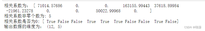
   establish the Lasso model to calculate the correlation coefficient, analyze and process the correlation coefficient, and get 5 non-zero correlation coefficients, which are the key factors affecting corporate income tax: the added value of the secondary industry (x1), the city Commodity retail price index (x4), total profit of construction enterprises (x5), loss of state-owned and state-holding industrial enterprises above designated size (x6), retail sales of chain stores (companies) above designated size (x9).

Fourth, training 3

#企业所得税灰色预测
import numpy as np
import pandas as pd
from GM11 import GM11 #引入自编的灰色预测函数

#数据抽取
inputfile = '../tmp/income_tax_deal.csv' #输入的数据文件
inputfile1 =  '../data/income_tax.csv' #输入的原数据文件 
new_income_tax = pd.read_csv(inputfile) # 读取经过特征选择后的数据
data = pd.read_csv(inputfile1) #读取总的数据
#预处理
new_income_tax.index = range(2004, 2016)
new_income_tax.loc[2014] = None
new_income_tax.loc[2015] = None
l = ['x1', 'x4','x5','x6','x9']  
for i in l:
    #as_matrix自0.23.0起不推荐使用该方法，因此应to_numpy改为使用
    f = GM11(new_income_tax.loc[range(2004,2014),i].to_numpy())[0] 
    new_income_tax.loc[2014,i] = f(len(new_income_tax)-1) #2014预测结果
    new_income_tax.loc[2015,i] = f(len(new_income_tax)) #2015预测结果
    new_income_tax[i] = new_income_tax[i].round(2)
outputfile = '../tmp/income_tax.csv_deal_GM11.xls'  #灰色预测后保存的路径
y = list(data['y'].values)
new_income_tax['y'] = y
new_income_tax.to_excel(outputfile,engine='openpyxl')
print('预测结果为：',new_income_tax.loc[2014:2015,:])

   Import the gray prediction function, read the data set that has undergone feature selection in the previous step, and use the gray prediction function to process it to establish a gray prediction model.

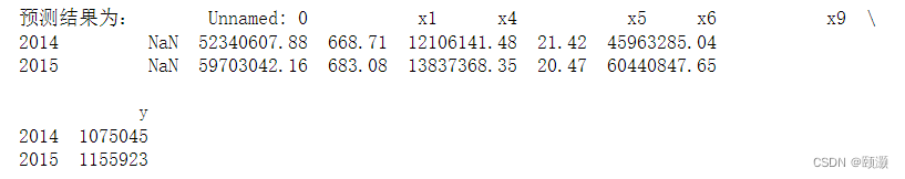
   From the above results, it can be clearly seen that the accuracy of the gray prediction is very high, and the predictions of x1, x4, x5, x6, and x9 in 2014 and 2015 are relatively accurate, laying a solid foundation for the following support vector regression prediction. Relatively good data basis, and the forecast of corporate income tax in 2014 and 2015 is very accurate.

vector regression model

   Substitute the results of the gray forecast in the previous step into the vector regression forecast model established by the corporate income tax

#企业所得税支持向量回归预测模型
import numpy as np;
import pandas as pd;
from sklearn.svm import LinearSVR
import matplotlib.pyplot as plt
from sklearn.metrics import explained_variance_score,mean_absolute_error, mean_squared_error,median_absolute_error,r2_score
inputfile = '../tmp/income_tax.csv_deal_GM11.xls' #灰色预测后保存的路径
data = pd.read_excel(inputfile) #读取数据
feature = ['x1', 'x4','x5','x6','x9'] 
data_train = data.loc[0:11,:]                                
data_mean = data_train.mean()
data_std = data_train.std()
data_train = (data_train - data_mean)/data_std                 #将数据数据标准化
x_train = data_train[feature].values                           #特征数据
y_train = data_train['y'].values                               #标签数据
linearsvr = LinearSVR()                                        #调用LinearSVR()函数
linearsvr.fit(x_train,y_train)
x = ((data[feature] - data_mean[feature])/ data_std[feature]).values      #进行预测，并还原结果。
data[u'y_pred'] = linearsvr.predict(x) * data_std['y'] + data_mean['y']
## SVR预测后保存的结果
outputfile = '../tmp/income_tax_corr_GM11_SVR.xls'
data.to_excel(outputfile,engine='openpyxl')
data.index = range(2004,2016)
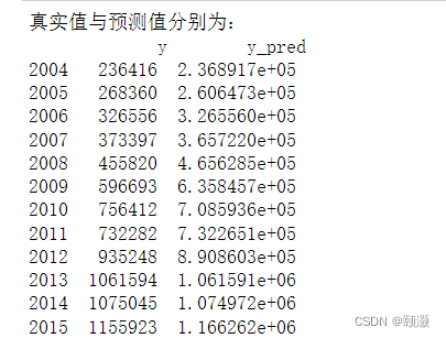
print('真实值与预测值分别为：','\n',data[['y','y_pred']])

print('预测图为：',data[['y','y_pred']].plot(subplots = True,
     style=['b-o','r-*'],xticks=data.index[::2]))

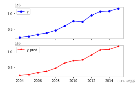
   From the above results and forecast chart, it can be clearly seen that the predicted value is very close to the real value, and the model's forecast of corporate income tax in 2014 and 2015 is accurate.

(5) Model evaluation

print('企业所得税回归模型的平均绝对误差为：',
      mean_absolute_error(data['y'].iloc[0:11],data['y_pred'].iloc[0:11]))
print('企业所得税回归模型的均方误差为：',
     mean_squared_error(data['y'].iloc[0:11],data['y_pred'].iloc[0:11]))
print('企业所得税回归模型的中值绝对误差为：',
     median_absolute_error(data['y'].iloc[0:11],data['y_pred'].iloc[0:11]))
print('企业所得税回归模型的可解释方差值为：',
     explained_variance_score(data['y'].iloc[0:11],data['y_pred'].iloc[0:11]))
print('企业所得税回归模型的R方值为：',
     r2_score(data['y'].iloc[0:11],data['y_pred'].iloc[0:11]))

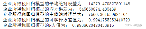
  From the above evaluation results, it can be concluded that the mean absolute error and the median absolute error are small, and the explainable variance value and the R square value are very close to 1, indicating that the established support vector regression model has a good fitting effect and can be used for corporate income taxation. Prediction.