Python analysis of second-hand housing data in Hangzhou
The data set comes from the public data on the Internet, python language, in terms of data analysis, as a sharp tool, it covers every link in the process of "data acquisition → data processing → data analysis → data visualization".
Environment construction:
Environment: win10+Anaconda +jupyter Notebook
Libraries: Numpy, pandas, matplotlib, seaborn, missingno, the management and installation of various packages mainly use conda and pip.
Dataset: Hangzhou second-hand housing information sample
Explore questions:
The questions to be explored are: 1. Regional location characteristics of second-hand housing 2. The proportion of the number of houses in the equal distance of the total price, the average value of the total price in each region 3. The proportion of the number of houses in the equal distance of the unit price, and the proportion of the unit price in each region 4. Visualization of viewing time 6. Analysis of attention characteristics 7. Floor height analysis 8. House type structure analysis 9. Building type 10. Orientation analysis 11. Building structure 12. Whether there is an elevator analysis 13. Use analysis 14. Core Selling point word cloud analysis
# Import the required database
import pandas as pd
import numpy as np
import seaborn as sns
sns.set()
import matplotlib.pyplot as plt
#
Set the configuration to output high-definition vector graphics:
%config InlineBackend.figure_format = 'svg'
%matplotlib
inline
# Use pandas to read and analyze data:
house = pd.read_csv("C:/Users/EVILLIFES/Desktop/Order Receiving/Secondhand_house.csv",encoding='gbk')
#
Output main information:
house.info( )
<class 'pandas.core.frame.DataFrame'>
RangeIndex: 8121 entries, 0 to 8120
Data columns (total 45 columns):
 # Column Non-Null Count Dtype
--- ------ ------ -------- -----
 0 serial number 8121 non-null int64
 1 community name 8121 non-null object
 2 area location 8121 non-null object
 3 longitude 8121 non-null object
 4 latitude 8121 non-null object
 5 total price 8121 NON-NULL Object
 6 Single price 8121 Non-Null Object
 7 Viewing time 8121 Non-Null Object
 8 Chain Home No. 8121 NON-NULL Object
 9 Following 8121 NON-NULL Object
 10 House Unit 8119 NON-NULL O Bject
 11 Floor 8121 non-null object
 12 architecture Area 8121 non-null object
 13 House type structure 7762 non-null object
 14 House area 8119 non-null object
 15 Building type 7762 non-null object
 16 House orientation 8121 non-null object
 17 Building structure 8119 non-null object
 18 Decoration condition 8119 non-null object
 19 Elevator ratio 7762 non-null object
 20 Equipped with elevator 7762 non-null object
 21 Listing time 8121 non-null object
 22 Transaction ownership 8121 non-null object
 23 Last transaction 8121 non-null object
 24 House purpose 8121 non-null object
 25 House years 8121 non-null object
 26 Ownership of property 8121 non-null object
 27 Mortgage information 8121 non-null object
 28 House book spare parts 8121 non-null object
 29 Uniform code for property verification 8121 non-null object
 30 Inquiry on record of housing management 7744 non-null object
 31 Core selling point 7747 non-null object
 32 Community introduction 5199 non-null object
 33 Peripheral supporting facilities 4958 non-null object
 34 Tax and fee analysis 821 non- null object
 35 Water type 1248 non-null object
 36 Electricity type 1248 non-null object
 37 Gas price 384 non-null object
 38 House type introduction 2390 non-null object
 39 Suitable crowd 1436 non-null object
 40 Decoration description620 non-null object
 41 Sales details 354 non-null object
 42 Transportation 200 non-null object
 43 Villa type 358 non-null object
 44 Ownership mortgage 21 non-null object
dtypes: int64(1), object(44)
memory usage: 2.8+ MB
# Get the number of rows and columns
rows = len(house)
columns = len(house.columns)
print(rows,columns)
# output column data type
columns_type = house.dtypes
columns_type
8121 45
Serial number int64
community name object
area location
object
longitude object latitude object
total price object unit
price object
viewing time object
home link number object
attention degree object
house type
object floor
object building area object
house type
structure object suite inner area object
building type object
house orientation object
building structure objectdecoration
condition objectelevator
ratio object
equipped with elevator
objectlisting time objecttransaction
ownership objectlast
transaction
objecthousing use
objecthousing age object
Property ownership objectmortgage
information objectproperty
spare parts objecthousing
verification uniform code objectinquiry
housing management records objectcore
selling point
objectcommunity introduction objectsurrounding facilities
objecttax
analysis objectwater
type objectelectricity
type objectgas
price objecthouse
type introduction objectsuitable
crowd object
Decoration descriptionobjectSales
details objectTraffic
travel objectVilla
type objectOwnership
mortgage object
dtype: object
# To display Chinese
from pylab import mpl
mpl.rcParams['font.sans-serif'] = [u'SimHei']
mpl.rcParams['axes.unicode_minus'] = False
# Through the above info information, we found that there are missing values in the data. Here we count the missing situations: missing_values = house.isnull().sum() print(missing_values) # Visually displayed as: import missingno as msno msno.matrix( house, figsize = (15,5), labels=True)
Serial number
0Community name 0Regional
location 0Longitude
0Latitude
0Total
price 0Unit
price 0Viewing
time 0Link
home number 0Attention 0House
type
2Floor 0Building
area
0House
type structure 359
sets of internal area 2Building
type 359Housing
orientation
0Building Structure 2Decoration
status 2Elevator
household ratio 359Elevator
359Listing
time 0Transaction
ownership 0Last
transaction 0House
purpose 0House
years 0Property
ownership 0Mortgage
information 0
Spare parts of the house 0Uniform
code for property verification 0Enquiry
of record of housing management 377Core selling
points 374Introduction
of community 2922Surrounding
facilities 3163Analysis
of taxes and fees 7300Type of
water 6873Type of
electricity 6873Gas
price 7737Introduction of house type
5731Suitable crowd 6685Description of
decoration
7501Details
of sales 7767
Transportation 7921
Villa Type 7763
Ownership Mortgage 8100
dtype: int64
<Axes: >
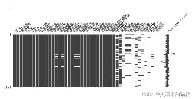
msno.bar(house,figsize = (15,5)) # bar graph display
<Axes: >

Data cleaning:
The data processing in this step is mainly the data set problem we found in the previous step: missing value problem. In actual business, data cleaning is often more troublesome than this. It is a complicated and cumbersome job (everyone who has used excel to clean data knows~). I saw on the Internet that some people say that 80% of the time for an analysis project is It is not unreasonable to clean the data. There are two purposes of cleaning. The first is to make data available through cleaning. The second is to make the data more suitable for subsequent analysis. In general, a "dirty" data should be clear, and a "clean" data should also be cleaned.
""Dirty" data needs to be cleaned, which is well known. But "clean" data also needs to be cleaned? This sounds very confusing. In fact, I personally think that the more accurate expression is that this belongs to the feature construction in feature engineering. Construct the features we need, which is conducive to the next step of analysis.
Take the data analysis clock as an example of our common problem of dealing with date variables. Sometimes we need to extract the corresponding week number from the date variable and construct it to express the date in the form of a week. Sometimes we need to extract the month from the date variable. , structured to display dates in months, or to discretize continuous numerical data, construct classification intervals, and so on. These processing methods are called feature engineering in ML, but they are essentially data cleaning.
In missing value processing, we generally delete missing values. In the pandas module, the method dropna() is provided to delete rows containing NaN values, but in fact, the best way to deal with missing values is to "replace it with the closest data"
For numerical data, it can be replaced by the mean or median of the data in the column. For categorical data, it can be filled with the most frequently occurring data (mode) of the data in the column.
If you really can't handle the null value, you can leave it temporarily, and don't worry about deleting it. Because it may appear in subsequent situations: subsequent operations can skip the null value.
Through the analysis of the null value data, we found that:【House type, type structure, apartment area, building type, building structure, decoration, ratio of elevators, equipped with elevators, query housing management records, core selling points, community introduction, surrounding facilities , tax and fee analysis, water type, electricity type, gas price, house type introduction, suitable crowd, decoration description, house sales details, transportation, villa type, and ownership mortgage] There is a loss of value.
The data that have an impact on the data we need are [family structure (missing 359), building type (missing 359), building structure (missing 2), equipped with elevators (missing 359), core selling points (missing 374), villa type (missing 7763 )].
We found that in these data, there is no column like a value, so we can skip missing values.
# Convert the total price and unit price columns to numeric types:
price = pd.to_numeric(house['total price'], errors='coerce',).fillna(0)
unit_price = pd.to_numeric(house['unit price'] , errors='coerce',).fillna(0)
print(price)
print(unit_price)
0 930.0
1 765.0
2 225.0
3 148.0
4 130.0
        ...
8116 205.0 8117 570.0
8118 440.0
8119
242.0
8120 325.0
Name: Total, Length: 8121, dtype: float64
0 69053.0
1
55423.0 2 34611.0
3 31835.0
4 26461.0
         ...
8116 30308.0
8117 36562.0
8118 48993.0
8119 32903.0
8120 44260.0
Name: unit price, Length: 8121, dtype: float64
# Total price analysis:
price.describe()
count 8121.000000
mean 429.089820
std 368.176619
min 0.000000
25% 210.000000
50% 320.000000
75% 545.000000
max 6500.000000
Name: total price, dtype: float64
# Unit price analysis:
unit_price.describe()
count 8121.000000
mean 40310.525305
std 18436.762039
min 0.000000
25% 26552.000000
50% 37487.000000
75% 48544.000000
max 128968.0000 00
Name: unit price, dtype: float64
#Fill the data of a column of building structure
# First check the current proportion
house['building structure'].value_counts()
Steel-concrete structure 5612
Brick-concrete structure 1015
Mixed structure 851
Frame structure 478
Steel structure 91
Unknown structure 44
Brick-wood structure 27
Building structure 1
Name: building structure, dtype: int64
# It is found that the steel-concrete structure accounts for the largest proportion, so we use the steel-concrete structure to supplement the missing value
house.fillna({'building structure':'steel-concrete structure'},inplace=True)
structure = house['building structure']
# Check if there are still missing values
structure.isnull().sum()
0
Handling of other missing values: In the pandas module, the method dropna() is provided to delete rows containing NaN values
data visualization
The pandas.pivot_table function contains four main variables, as well as some optional parameters. The four main variables are data source data, row index index, columns columns, and numerical values. Optional parameters include how values are summarized, how NaN values are handled, and whether to display summary row data.
In terms of visual analysis, it will involve python's commonly used drawing libraries: matplotlib and seaborn. There are already a lot of user guides on the Internet, so I won't say much here. I will make some summaries when I have time in the future.
#Manual interval division
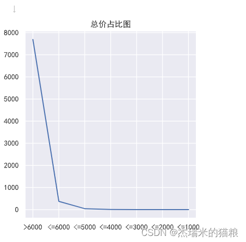
# Total price ratio:
f1 = [0,0,0,0,0,0,0]
y1 = ['>6000','<=6000','<=5000','<= 4000','<=3000','<=2000','<=1000']
for i in price:
if i<=1000.0:
f1[0]+=1
elif i<=2000.0:
f1[1]+ =1
elif i<=3000.0:
f1[2]+=1
elif i<=4000.0:
f1[3]+=1
elif i<=5000.0:
f1[4]+=1
elif i<=6000.0:
f1[5 ]+=1
else:
f1[6]+=1
print(f1)
plt.figure(figsize = (10,5))
plt.subplot(121) # The first subplot
plt.title("total price ratio plot")
plt.plot(y1,f1)
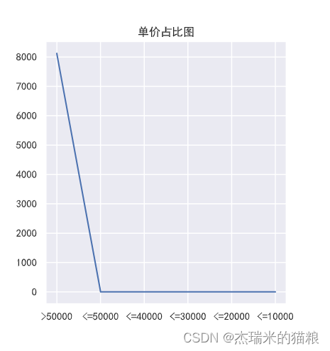
# unit price ratio:
f2 = [0,0,0,0,0,0]
y2 = ['>50000','<=50000','<=40000','<=30000','<=20000','<=10000'] for i in price: if i<=
10000.0
:
f2 [0]+=1
elif i<=20000.0:
f2[1]+=1
elif i<=30000.0:
f2[2]+=1
elif i<=40000.0:
f2[3]+=1
elif i<=50000.0 :
f2[4]+=1
else:
f2[5]+=1
print(f2)
plt.figure(figsize = (10,5))
plt.subplot(122) # first subplot
plt.title(" Unit price ratio chart")
plt.plot(y2,f2)
[7691, 373, 44, 8, 3, 1, 1]
[8121, 0, 0, 0, 0, 0]
[<matplotlib.lines.Line2D at 0x283bed15c30>]
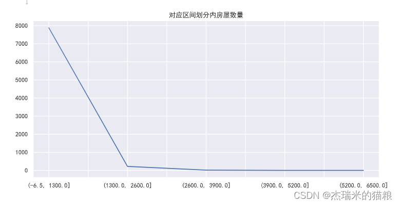
# Use tools to divide intervals
house["total price distribution"]=pd.cut(price,5)#Divide the value of the age column into 5 equal parts
price_info = house["total price distribution"].value_counts(sort=False )#Check how many people are in each group

price_info.plot(label='quantity', title='the number of houses in the corresponding interval division', figsize=(11,5))
plt.show()
# Regional unit price analysis
f3 = house['area location'].value_counts(ascending=True)
print(f3)
plt.figure(figsize= (25 ,5))#Create canvas
plt.xticks(rotation = 90) # Abscissa
plt.plot(f3, linewidth=3, marker='o',
         markerfacecolor='blue', markersize=5)

plt.title('Regional room statistics')
plt.show()
Regional Location 1
Fuyang 1
Gongshu - Jianqiao 22
Gongshu - Tianshui 24
Gongshu - Desheng East 24
Gongshu - Stadium Road 28
Gongshu - Sanli Pavilion 33
Gongshu - Silk City 34
Gongshu - Peace 39
Fuyang - Jiangnan New City 42
Gongshu-Wulin 43 Gongshu
-Wanda Plaza 50
Gongshu-Zhong'an Bridge 57
Gongshu-Desheng 74
Gongshu-Chaoming 85
Gongshu-Changqing 86
Gongshu-Sandun 87
Fuyang-Fuyang 91
Fuyang-Lushan New City 95
Gongshu-Hemu 111
Gongshu-Xinyifang 118
Gongshu-Hushu 128
Riverside-White Horse Lake 138
Gongshu-Daguan 153
Gongshu-Qiaoxi 160
Gongshu-Zhaohui 169
Gongshu-Mid-Levels 181
Gongshu-Jianguo North Road 186
Gongshu - Liushuiyuan 187
Gongshu-Shiqiao 187
Binjiang-Aoti 199
Binjiang-Xixing 209
Gongshu-Shenhua 238 Gongshu-Gongchen Bridge 239
Gongshu-
Santang 257 Binjiang-Changhe
335
Fuyang-Dongzhou 392
Fuyang-Fuchun 513
Binjiang- Puyan 554
Binjiang-Rainbow City 635
Binjiang-Binjiang District Government 930
Fuyang-Yinhu Science and Technology City 986
Name: Regional location, dtype: int64

We found that the unit price is generally higher in Binjiang District, while Fuyang-Silver Lake Science and Technology City is more expensive
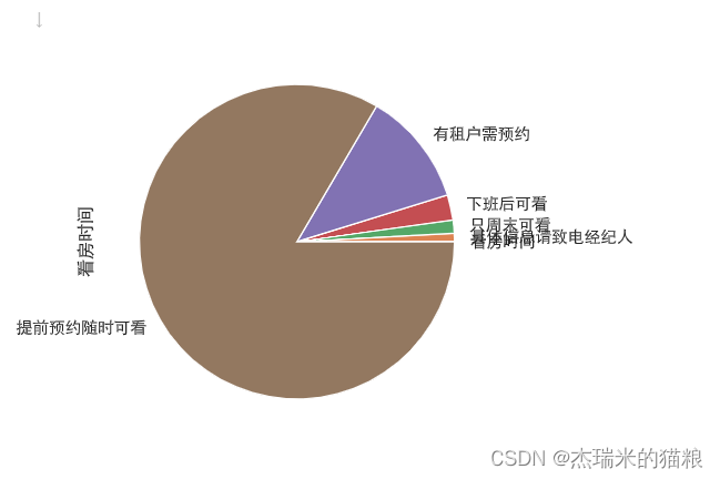
# Viewing time analysis
f4 = house['viewing time'].value_counts(ascending=True)
print(f4)
plt.figure(figsize= (9 ,5))#Create canvas
plt.xticks(rotation = 90) # Abscissa
plt.plot(f4, linewidth=3, marker='o',
         markerfacecolor='blue', markersize=5)
plt.title('Statistics of viewing time')
plt.show()
#Through the chart we found that, Most of the customers who look at the house choose to make an appointment in advance and watch it at any time.
Viewing time 1
For specific information, please call the broker 68
only on weekends, 111
after work, 210
, tenants need to make an appointment 955, make
an appointment in advance and view at any time 6776
Name: viewing time, dtype: int64

# Use a pie chart to view
print(type(f4))
f4.plot.pie()
<class 'pandas.core.series.Series'>
<Axes: ylabel='Viewing time'>
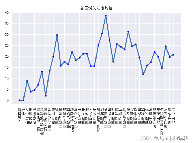
# The average degree of concern in each region:
house['concern'] = pd.to_numeric(house['concern'], errors='coerce',).fillna(0)
f5 = house.groupby('regional location' )['attention'].mean().to_dict()
print(f5)

x = list(f5.keys())
y = list(f5.values())
plt.figure(figsize= (9 ,5) )# Create canvas
plt.xticks(rotation = 90) # Abscissa coordinates
plt.plot(x, y, linewidth=3, marker='o',markerfacecolor='blue', markersize=5)

plt.title('Each area Attention average')
plt.show()
{'Regional Location': 0.0, 'Fuyang': 0.0, 'Fuyang-Dongzhou': 8.721938775510203, 'Fuyang-Fuchun': 3.9688109161793372, 'Fuyang-Fuyang': 4.758241758241758, 'Fuyang-Jiangnan New City': 7.07 1428571428571, ' Fuyang-Silver Lake Science and Technology City': 13.101419878296147, 'Fuyang-Lushan New City': 2.1052631578947367, 'Gongshu-Wanda Plaza': 13.44, 'Gongshu-Santang': 19.972762645914397, 'Gongshu-Sandun': 29.71 264367816092, ' Gongshu - Sanli Pavilion': 15.757575757575758, 'Gongshu - Silk City': 17.61764705882353, 'Gongshu - Zhong'an Bridge': 16.42105263157895, 'Gongshu - Stadium Road': 21.821428571428573, 'Gongshu - Xinyi Square': 18.347457627118644, 'Gongshu-Mishan': 19.41988950276243, 'Gongshu-Peace': 21.128205128205128, 'Gongshu-Harmony': 21.135135135135137, 'Gongshu-Daguan': 15.627450980392156, 'Gongshu-Tianshui' : 15.625, 'Gongshu- Jianguo North Road': 25.118279569892472, 'Gongshu-Desheng': 30.5, 'Gongshu-Desheng East': 38.541666666666664, 'Gongshu-Gongchen Bridge': 27.476987447698743, 'Gongshu-Zhaohui': 17.644970414201183, 'Gongshu-Qiaoxi': 25.625, 'Gongshu-Wulin': 24.348837209302324, 'Gongshu-Liushuiyuan': 23.11764705882353, 'Gongshu-Hushu': 31.3203125, 'Gongshu-Chaoming': 24.658823529411766, 'Gongshu-Shenhua': 25.449579831932773, 'Gongshu-Stone Bridge': 19.56149732620321, 'Gongshu-Jianqiao': 11.909090909090908, 'Gongshu- Changqing': 15.883720930232558, 'Binjiang -Olympic Sports': 17.417085427135678, 'Binjiang-Rainbow City': 21.973228346456693, 'Binjiang-Puyan': 19.862815884476536, 'Binjiang-Binjiang District Government': 14.706451612903226, 'Binjiang-White Horse Lake ': 24.579710144927535, 'Binjiang-Xixing' : 19.679425837320576, 'Binjiang-Changhe': 20.755223880597015}449579831932773, 'Gongshu-Stone Bridge': 19.56149732620321, 'Gongshu-Jianqiao': 11.909090909090908, 'Gongshu-Changqing': 15.883720930232558, 'Binjiang-Aoti': 17.4170 85427135678, 'Binjiang-Rainbow City': 21.973228346456693, ' Binjiang-Puyan': 19.862815884476536, 'Binjiang-Binjiang District Government': 14.706451612903226, 'Binjiang-White Horse Lake': 24.579710144927535, 'Binjiang-Xixing': 19.679425837320576, 'Binjiang -long river': 20.755223880597015}449579831932773, 'Gongshu-Stone Bridge': 19.56149732620321, 'Gongshu-Jianqiao': 11.909090909090908, 'Gongshu-Changqing': 15.883720930232558, 'Binjiang-Aoti': 17.4170 85427135678, 'Binjiang-Rainbow City': 21.973228346456693, ' Binjiang-Puyan': 19.862815884476536, 'Binjiang-Binjiang District Government': 14.706451612903226, 'Binjiang-White Horse Lake': 24.579710144927535, 'Binjiang-Xixing': 19.679425837320576, 'Binjiang -long river': 20.755223880597015}
# House type structure analysis
f6 = house['House type structure'].value_counts(ascending=True)
f6.plot.pie()
plt.title('House type structure analysis')
# The icons show that most of them are sold by square.
Text(0.5, 1.0, 'Household Structure Analysis')

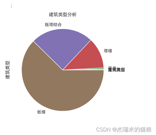
# Building type:
f7 = house['Building Type'].value_counts(ascending=True)
f7.plot.pie()
plt.title('Building Type Analysis')
# Icons represent mostly slab buildings
Text(0.5, 1.0, 'Building Type Analysis')
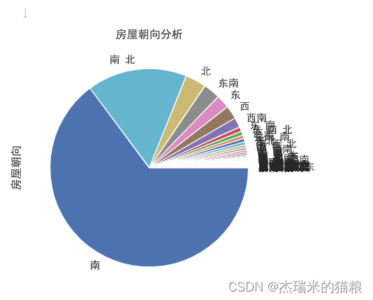
# House orientation:
f8 = house['House Orientation'].value_counts(ascending=True)
f8.plot.pie()
plt.title('House Orientation Analysis')
# Most of the faces are facing south
Text(0.5, 1.0, 'house orientation analysis')
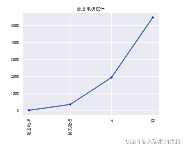
#Elevator equipped:
f9 = house['Elevator equipped'].value_counts(ascending=True)
print(f9)
plt.xticks(rotation = 90) # Abscissa coordinates
plt.plot(f9, linewidth=3, marker='o' ,
         markerfacecolor='blue', markersize=5)

plt.title('Statistics of equipped with elevators')
plt.show()
# The performance is mostly equipped with elevators
Equipped with elevator 1
No data yet 348
No 1937
Yes 5476
Name: Equipped with elevator, dtype: int64
# House use:
f10 = house['house use'].value_counts(ascending=True)
print(f10)
plt.xticks(rotation = 90) # Abscissa coordinates
plt.plot(f10, linewidth=3, marker='o' ,
         markerfacecolor='blue', markersize=5)

plt.title('Statistics of housing use')
plt.show()
# It shows that most of them are ordinary houses
Housing use 1
garage 2
villas 357
Commercial and residential use 1247
Ordinary residence 6514
Name: Housing use, dtype: int64

# Selling point core analysis
# Import word cloud library
import wordcloud # Import jieba library, use
import jieba
for word segmentation
# Accurate mode, return a list after word segmentation
ls = jieba.lcut(str(house['core selling point']))
# replace spaces Separated from word segmentation
txt1 = " ".join(ls)
w = wordcloud.WordCloud(font_path="simkai.ttf", background_color="white",
                        width=600, height=400, max_font_size=120, max_words=3000)
# Generate word cloud
w.generate(txt1)
# Name the word cloud image
w.to_file("maidian.png")
# Most of them show the characteristics of being close to the market, night market, convenient shopping, clean and so on