视觉SLAM十四讲学习记录 第四讲

之前第三讲的地址

第四讲 李群与李代数

  在第3讲中，我们介绍了三维世界中刚体运动的描述方式。并且在其中我们重点介绍了旋转的表示。不过在SLAM中，除了表示，我们还要对它们进行估计和优化。因为在SLAM中位姿是未知的，而我们需要解决形如“什么样的相机位姿最符合当前观测数据”这样的问题。一种典型的方式是把它构建成一个优化问题，求解最优的$R,t,$使得误差最小化。
  如前所言，旋转矩阵自身是带有约束的（正交且行列式为1）。它们作为优化变量时，会引入额外的约束，使优化变得困难。通过李群——李代数间的转换关系，我们希望把位姿估计变成无约束的优化问题，简化求解方式。

4.1 李群与李代数基础

  第3讲中，我们介绍了旋转矩阵和变换矩阵的定义。当时，我们说三维旋转矩阵构成了特殊正交群SO(3),而变换矩阵构成了特殊欧氏群SE(3)。它们写起来像这样：
          S O ( 3 ) = { R ∈ R 3 × 3 ∣ R R T = I , d e t ( R ) = 1 } SO(3) = \{R∈\mathbb{R}^{3 × 3}|RR^T = I,det(R) = 1\} SO(3)={ R∈R3×3∣RRT=I,d e t ( R )=1}
          S E ( 3 ) = { T = [ R t 0 T 1 ] ∈ R 4 × 4 ∣ R ∈ S O ( 3 ) , t ∈ R 3 } SE(3) = \{T=\begin{bmatrix}R&t\\\\0^T&1\end{bmatrix}∈\mathbb{R}^{4 × 4}|R ∈ SO(3),t ∈ \mathbb{R}^3\} SE ( 3 )={ T=⎣ ⎡​R0T​t1​⎦ ⎤​∈R4×4∣R∈SO(3),t∈R3 }
  However, we did not explaingroup. Readers should be able to notice that, whether it is a rotation matrix or a transformation matrix, **they are not closed to addition. **In other words, for any two rotation matrices$R_1,R_2,$ according to the definition of matrix addition, and is no longer a rotation matrix:

         $R_1+R_2\notin SO(3),T_1+T_2\notin SE\left(3\right).$

You could also say that there is no well-defined addition of two matrices, or that matrix addition in general is not closed over the two sets. Instead, they have only one nice operation: multiplication. $SO\left(3\right)$ sumSE$SE\left(3\right)$ is closed with respect to multiplication:

         $R_1{R}_2\in SO\left(3\right),T_1{T}_2\in SE\left(3\right).$

At the same time, we can also invert (in the sense of multiplication) any rotation or transformation matrix. We know that multiplication corresponds to the composition of rotation or transformation, and the multiplication of two rotation matrices means that two rotations have been performed. For such a collection with only one (good) operation, we call it a group .

4.1.1 Group

  Next, we need to introduce some knowledge of abstract algebra.
  Group (Group) is an algebraic structure of a set plus an operation . We denote the set as $A,$ the operation is denoted as$\cdot ,$ then the group can be recorded as$G=(A,\cdot ).$The group requires this operation to satisfy the following conditions:

1. 封闭性： $\forall a_1,a_2\in A,a_1\cdot a_2\in A.$
2. 结合律：$\forall a_1,a_2,a_3\in A,(a_1\cdot a_2)\cdot a_3=a_1\cdot (a_2\cdot a_3)$
3. 幺元：$\exists a_0\in A,s.t.\forall a\in A,a_0\cdot a=a\cdot a_0=a.$
4. 逆：$\forall a\in A,\exists a^{-1}\in A,s.t.a\cdot a^{-1}=a_0.$

  读者可以将上述四个性质记作“封结幺逆”。容易验证，旋转矩阵集合和矩阵乘法构成群，同样，变换矩阵和矩阵乘法也构成群（因此才能称它们为旋转矩阵群和变换矩阵群）。其他常见的群包括整数的加法$(\mathbb{Z},+),$去掉0后的有理数的乘法（幺元为1）$(\mathbb{Q}\setminus 0,\cdot ),$ and so on. Common groups in matrices are:

• General Linear Group $GL\left(n\right)$  指$n\times Invertible\; matrices\; of\; n$ that group for matrix multiplication.
• Special Orthogonal Group $SO\left(n\right)$  is the so-called rotation matrix group, where$SO\left(2\right)$ sum$SO\left(3\right)$ is the most common.
• Special Euclidean group $SE\left(n\right)$  is the aforementioned$n-$ dimensional Euclidean transformation, such as$SE\left(2\right)$ SumSE$SE\left(3\right)$。

  The group structure ensures that the operations on the group have good properties, and the group theory is the theory of studying various structures and properties of the group. Readers interested in group theory can refer to any modern algebra textbook. A Lie group is a group that has the continuous (smooth) property. Like the integer group Z \mathbb{Z}A discrete group like$Z\; has\; no\; continuous\; property,\; so\; it\; is\; not\; a\; Lie\; group.$while$SO\left(n\right)$ sumSE$SE\left(n\right)$ is continuous in the space of real numbers. We can intuitively imagine that a rigid body can move continuously in space, so they are all Lie groups. Since$SO\left(3\right)$ sumSE$SE\left(3\right)$ is especially important for camera pose estimation, so we mainly discuss these two Lie groups. Then from the simpler$SO\left(3\right)$ starts the discussion leading toSO ( 3 ) SO (3)The Lie algebra above$SO$$($$3$$)$$\mathfrak{so}(3)$

4.1.2 Derivation of Lie algebra

  Consider any rotation matrix $R,$ we know it satisfies:

         $R{R}^T=I$

Now, we say, $R$ is the rotation of some camera, which changes continuously over time, as a function of time:$R\left(t\right).$Since it is still a rotation matrix, there is

         $R(t)R(t{)}^T=I$

Taking the derivative with respect to time on both sides of the equation, we get

         $\dot{R}(t)R(t{)}^T+R(t)\dot{R}(t{)}^T=0$

Tidy up

         $\dot{R}(t)R(t{)}^T=-(\dot{R}\left(t\right)R(t{)}^T{)}^T$

  It can be seen that $\dot{R}\left(t\right)R(t{)}^T$ is anantisymmetric matrix. When introducing the cross product before, the ^ symbol was introduced to turn a vector into an anti-symmetric matrix. Similarly, for any anti-symmetric matrix, we can also find the only corresponding vector, and use this operation symbol$\stackrel{ˇ}{}$ said:

         $a^{\wedge }=A=\left[\begin{array}{ccc}0& -a_3& a_2\\ & & \\ a_3& 0& -a_1\\ & & \\ -a_2& a_1& 0\end{array}\right],A^{\vee }=a$

  于是，由于$\dot{R}(t)R(t{)}^T$是一个反对称矩阵，我们可以找到一个三维向量$\varphi (t)\in {\mathbb{R}}^3$与之对应：

         $\dot{R}(t)R(t{)}^T=\varphi (t{)}^{\wedge }.$

  等式两边右乘$R(t),$由于$R$为正交阵，有

         $\dot{R}(t)=\varphi (t{)}^{\wedge }R(t)=\left[\begin{array}{ccc}0& -{\varphi }_3& {\varphi }_2\\ & & \\ {\varphi }_3& 0& -{\varphi }_1\\ & & \\ -{\varphi }_2& {\varphi }_1& 0\end{array}\right]R(t).$

  It can be seen that to obtain a derivative for each pair of rotation matrices, just multiply by a ${\varphi }^{\wedge }\left(t\right)$matrix is ​​enough. Consider$t_0=When\; 0$ , set the rotation matrix at this time as$R(0)=I.\_$According to the definition of derivative, we can put$R\left(t\right)$ at$t=$Perform a first-order Taylor expansion around$0\; :$

         $\begin{array}{rl}R(t)& \approx R(t_0)+\dot{R}(t_0)(t-t_0)\\ & =I+\varphi (t_0{)}^{\wedge }(t).\end{array}$

  We see that $\varphi$ reflectsthe RRThe derivative property of$R$$SO\left(3\right)$ on the Tangent Space near the origin. At the same time at$t_0$Nearby, let $\varphi$ remains constant$\varphi (t_0)={\varphi }_0.$Therefore:

         $\dot{R}(t)=\varphi (t_0{)}^{\wedge }R(t)={\varphi }_0^{\wedge }R(t).$

  The above formula is about $Differential\; equation\; of\; R$ with initial value$R(0)=I$ , solved

         $R(t)=\exp ({\varphi }_0^{\wedge }t).$

  The reader can verify that the above formula holds for both differential equations and initial values. This means that at $t=Near\; 0$ , the rotation matrix can be calculated by$\exp \left({\varphi }_0^{\wedge }t\right)$ is calculated. We see that the rotation matrix$R$ and another antisymmetric matrix${\varphi }_0^{\wedge }t$ is connected through an exponential relationship. But what is the index of the matrix? Here we have two questions to clarify:

1. Given $R,$ we can find a$\varphi ,$ which describes$R$ in the local derivative relationship. with$R$ corresponds toϕ \phiWhat does$\varphi \; mean?$We say that$\varphi$ exactly corresponds toSO ( 3 ) SO(3)Lie algebra on$SO$$($$3$$)$$\mathfrak{so}(3);$
2. Second, given a certain vector $\varphi$ , matrix exponent$\exp \left({\varphi }^{\wedge }\right)$how to calculate? Conversely, given$In\; R$ , can there be an inverse operation to calculate$\varphi ?$ In fact, this is exactly the exponential/logarithmic mapping between Lie groups and Lie algebras.

  Below, we address these two issues.

4.1.3 Definition of Lie algebra

  Every Lie group has a corresponding Lie algebra. Lie algebras describe the local properties of Lie groups, to be precise, the tangent space around the identity element. A general Lie algebra is defined as follows:
  Lie algebra consists of a set $V,$ a number field$F$ and a binary operation$[,]$组成。如果它们满足以下几条性质，则称$(\mathbb{V},\mathbb{F},[,])$为一个李代数，记作$\mathfrak{g}。$

1. 封闭性 $\forall X,Y\in \mathbb{V},[X,Y]\in \mathbb{V}.$
2. 双线性 $\forall X,Y,Z\in \mathbb{V},a,b\in \mathbb{F},$有
            $[aX+bY,Z]=a[X,Z]+b[Y,Z],[Z,aX+bY]=a[Z,X]+b[Z,Y].$
3. 自反性 $\forall X\in \mathbb{V},[X,X]=0.$
4. 雅可比等价 $\forall X,Y,Z\in \mathbb{V},[X,[Y,Z]]+[Z,[X,Y]]+[Y,[Z,X]]=0$

where binary operations are called Lie brackets . On the surface, Lie algebras need quite a lot of properties. In contrast to the simpler binary operations in groups, Lie brackets express the difference between two elements. It does not require the associative law, but requires the property that the element and itself are zero after the braces. As an example, the three-dimensional vector ${\mathbb{R}}^{}$The cross product × defined on${}^3$$\mathfrak{g}=({\mathbb{R}}^3,\mathbb{R},\times )$ form a Lie algebra.

4.1.4 Lie algebra $\mathfrak{so}(3)$

  The previously mentioned $\varphi ,$ is in fact a Lie algebra. $SO\left(3\right)$ corresponds to the definition in${\mathbb{R}}^{}$The vector on${}^3$$\varphi$ . According to the previous derivation, each$\varphi$ can generate an antisymmetric matrix:

         $Phi={\varphi }^{\wedge }=\left[\begin{array}{ccc}0& -{\varphi }_3& {\varphi }_2\\ & & \\ {\varphi }_3& 0& -{\varphi }_1\\ & & \\ -{\varphi }_2& {\varphi }_1& 0\end{array}\right]\in R^{3\times 3}.$
  Under this definition, two vectors${\varphi }_1,{\varphi }_2$The braces for

         $[p_1,{\varphi }_2]=(F_1{Phi}_2-{Phi}_2{Phi}_1{)}^{\vee }.$

  Readers can verify whether the braces under this definition satisfy the above four properties. Since the vector $There\; is\; a\; one-to-one\; correspondence\; between\; \varphi$ and anti-symmetric matrix,$The\; elements\; of\; so\left(3\right)$ are three-dimensional vectors or three-dimensional antisymmetric matrices, without distinction:

         $\mathfrak{so}(3)=\{p\in {\mathbb{R}}^3,Phi={\varphi }^{\wedge }\in R^{3\times 3}\}.$

Some books also use $\hat{\varphi }$Such a notation indicates anti-symmetry, but the meaning is the same. So far, we have cleared $the\; content\; of\; so\left(3\right)$ . They are athree-dimensional vector, each corresponding to an antisymmetric matrix, which can be used to express the derivative of the rotation matrix. It is related to$SO\left(3\right)$ the relation is given by an exponential map:

         $R=\exp ({\varphi }^{\wedge }).$

Exponent mappings are covered later. Since so ( 3 ) has been introduced $so\left(3\right),$ let's take a look atSE ( 3 ) SE(3)The Lie algebra corresponding to$SE$$($$3$$)\; .$

4.1.5 Lie algebra $with\left(3\right)$

  For $SE\left(3\right)$ also has a corresponding Lie algebra$se\left(3\right).$In order to save space, how to introduce$se\left(3\right)$ . with$so\left(3\right)$ is similar,$se\left(3\right)$ is located at${\mathbb{R}}^6$ spaces:

         $with\left(3\right)=\left\{X=\left[\begin{array}{c}r\\ \\ \end{array}\right]\in {\mathbb{R}}^6,r\in R^3,\varphi \in \mathfrak{so}(3),X^{\wedge }=\left[\begin{array}{cc}{\varphi }^{\wedge }& r\\ & \\ 0^T& 0\end{array}\right]\in R^{4\times 4}\right\}.$

We take each $The\; elements\; of\; se\left(3\right)$ are denoted as$\xi ,$ which is a six-dimensional vector. The first three dimensions are translation, denoted as$\rho ;$ the last three dimensions are rotations, denoted as$\varphi ,$ which is essentially$so\left(3\right)$ elements. At the same time, we extended$\stackrel{The\; meaning\; of\; the\; ˆ}{}$ symbol. at$se\left(3\right)$ , also use$\stackrel{ˆ}{}$ symbol, converts a six-dimensional vector into a four-dimensional matrix, but here no longer expresses anti-symmetry:

         $X^{\wedge }=\left[\begin{array}{cc}{\varphi }^{\wedge }& r\\ & \\ 0^T& 0\end{array}\right]\in {\mathbb{R}}^{4\times 4}.$

  We still use $\stackrel{ˆ}{}$ 和$\stackrel{ˇ}{}$ 符号指代“从向量到矩阵”和“从矩阵到向量”的关系，以保持和$\mathfrak{so}(3)$上的一致性。它们依旧是一一对应的。读者可以简单地把$\mathfrak{se}(3)$理解成“由一个平移加上一个$\mathfrak{so}(3)$元素构成的向量”（尽管这里的$\rho$还不直接是平移）。同样，李代数$\mathfrak{se}(3)$也有类似于$\mathfrak{so}(3)$的李括号：

         $[{\xi }_1,{\xi }_2]=({\xi }_1^{\wedge }{\xi }_2^{\wedge }-{\xi }_2^{\wedge }{\xi }_1^{\wedge }{)}^{\vee }.$

  读者可以验证它是否满足李代数的定义。至此，我们已经见过两种重要的李代数$\mathfrak{so}(3)$和$\mathfrak{se}(3)$了。

4.2 指数与对数映射

4.2.1 $SO(3)$上的指数映射

  现在来考虑第二个问题：如何计算$\exp ({\varphi }^{\wedge })?$显然它是一个矩阵的指数，在李群和李代数中，称为指数映射（Exponential Map）。同样，我们会先讨论 s o ( 3 ) \mathfrak{so}(3) The exponential map of$so$$($$3$$)$$se\left(3\right)$ situation.
  The exponential map of any matrix can be written as a Taylor expansion, but only if it converges, the result is still a matrix:

         $\exp (A)=\sum _{n=0}^{\infty }\frac{1}{n!}{A}^n.$

  Similarly, for so ( 3 ) \mathfrak{so}(3)Any element in$so$$($$3$$)$$\varphi ,$ we can also define its exponential map in this way:

         $\exp ({\varphi }^{\wedge })=\sum _{n=0}^{\infty }\frac{1}{n!}({\varphi }^{\wedge }{)}^n.$

但这个定义没法直接计算，因为我们不想计算矩阵的无穷次幂。下面我们推导一种计算指数映射的简便方法。由于$\varphi$是三维向量，我们可以定义它的模长和方向，分别记作$\theta$和$a，$于是有$\varphi =\theta a。$这里$a$是一个长度为1的方向向量，即$\Vert a\Vert =1。$首先，对于$a^{\wedge },$有以下两条性质：

         $a^{\wedge }{a}^{\wedge }=\left[\begin{array}{ccc}-a_2^2-a_3^2& a_1{a}_2& a_1{a}_3\\ & & \\ a_1{a}_2& -a_1^2-a_3^2& a_2{a}_3\\ & & \\ a_1{a}_3& a_2{a}_3& -a_1^2-a_2^2\end{array}\right]=a{a}^T-I,$

  as well as

         $a^{\wedge }{a}^{\wedge }{a}^{\wedge }=a^{\wedge }(a{a}^T-I)=-a^{\wedge }.$

These two formulas provide the processing $a^{\wedge }$ methods for higher-order terms. We can write the exponential map as

         $\begin{array}{rl}\exp ({\varphi }^{\wedge })=\exp \left(\theta a^{\wedge }\right)& =\sum _{n=0}^{\infty }\frac{1}{n!}(i{a}^{\wedge }{)}^n\\ & =I+i{a}^{\wedge }+\frac{1}{2!}{i}^{2a}{\_}^{\wedge }{a}^{\wedge }+\frac{1}{3!}{i}^3{a}^{\wedge }{a}^{\wedge }{a}^{\wedge }+\frac{1}{4!}{i}^4(a^{\wedge }{)}^4+\cdot \cdot \cdot \\ & =a{a}^T-a^{\wedge }{a}^{\wedge }+i{a}^{\wedge }+\frac{1}{2!}{i}^{2a}{\_}^{\wedge }{a}^{\wedge }-\frac{1}{3!}{i}^3{a}^{\wedge }-\frac{1}{4!}{i}^4(a^{\wedge }{)}^2+\cdot \cdot \cdot \\ & =a{a}^T+\begin{array}{c}\underbrace{(i-\frac{1}{3!}{i}^3+\frac{1}{5!}{i}^5-\cdot \cdot \cdot )}\\ \sin \end{array}{a}^{\wedge }-\begin{array}{c}\underbrace{(1-\frac{1}{2!}{i}^2+\frac{1}{4!}{i}^4-\cdot \cdot \cdot )}\\ \cos \end{array}{a}^{\wedge }{a}^{\wedge }\\ & =a^{\wedge }{a}^{\wedge }+I+\sin i{a}^{\wedge }-\cos i{a}^{\wedge }{a}^{\wedge }\\ & =(1-\cos i)a^{\wedge }{a}^{\wedge }+I+\sin i{a}^{\wedge }\\ & =\cos \theta I+(1-\cos \theta )a{a}^T+\sin \theta a^{\wedge }\end{array}$

  最后，得到一个似曾相识的式子：

         $\exp (\theta a^{\wedge })=\cos \theta I+(1-\cos \theta )a{a}^T+\sin \theta a^{\wedge }.$

  回想第3讲的内容，它和罗德里格斯公式如出一辙。这表明，$\mathfrak{so}(3)$实际上就是由所谓的旋转向量组成的空间，而指数映射即罗德里格斯公式。通过它们，我们把$\mathfrak{so}(3)$中任意一个向量对应到了一个位于$SO(3)$中的旋转矩阵。反之，如果定义对数映射，也能把$SO(3)$中的元素对应到$\mathfrak{so}(3)$中：

         $\varphi =\ln (R{)}^{\vee }={\left(\sum _{n=0}^{\infty }\frac{(-1{)}^n}{n+1}(R-I{)}^{n+1}\right)}^{\vee }.$

和指数映射一样，我们没必要直接用泰勒展开计算对数映射。在第3讲中，我们介绍过如何根据旋转矩阵计算对应的李代数，利用迹的性质分别求解转角和转轴，采用这种方式更省事。
  现在，我们介绍了指数映射的计算方法。那么，指数映射有何性质呢？是否对于任意的$R$都能找到一个唯一的$\varphi ?$很遗憾，指数映射只是一个满射，并不是单射（有关满射、单射、双射参考图灵的猫i的文章）。这意味着每个$SO(3)$中的元素，都可以找到一个$\mathfrak{so}(3)$元素与之对应；但是可能存在多个$\mathfrak{so}(3)$中的元素，对应到同一个$SO(3)$。至少对于旋转角$\theta$，我们知道多转$360°$ is the same as no rotation - it has periodicity. However, if we fix the rotation angle at$\pm \pi$ , then there is a one-to-one correspondence between Lie groups and Lie algebra elements.
  $SO\left(3\right)$ and$The\; conclusion\; of\; so\left(3\right)$ seems to be within our expectations. It is very similar to the rotation vector and rotation matrix we talked about earlier, and the exponential map is the Rodriguez formula. The derivative of a rotation matrix can be specified by a rotation vector, which guides how to perform calculus operations on rotation matrices.

4.2.2 SE ( 3 ) SE(3)Exponential mapping on$SE$$($$3$$)$

  The following introduces se ( 3 ) \mathfrak{se}(3)Exponential map on$se$$($$3$$)\; .$As above, the form is as follows:

         $\begin{array}{rl}\exp ({\xi }^{\wedge })& =\left[\begin{array}{cc}\sum _{n=0}^{\infty }\frac{1}{n!}({\varphi }^{\wedge }{)}^n& \sum _{n=0}^{\infty }\frac{1}{(n+1)!}({\varphi }^{\wedge }{)}^n\rho \\ & \\ 0^T& 1\end{array}\right]\\ & \\ & \stackrel{\Delta }{=}\left[\begin{array}{cc}R& Jp\\ & \\ 0^T& 1\end{array}\right]=T\end{array}$

  只要有一点耐心，可以照着$So\left(3\right)$ derivation, put$\exp$ conducts a Taylor expansion to derive the matter. Let$\varphi =\theta a,$ where$a$ is a unit vector, then

         $\begin{array}{rl}\sum _{n=0}^{\infty }\frac{1}{(n+1)!}({\varphi }^{\wedge }{)}^n& =I+\frac{1}{2!}i{a}^{\wedge }+\frac{1}{3!}{i}^2(a^{\wedge }{)}^2+\frac{1}{4!}{i}^3(a^{\wedge }{)}^3+\frac{1}{5!}{i}^4(a^{\wedge }{)}^4\cdot \cdot \cdot \\ & =\frac{1}{i}\begin{array}{c}(\frac{1}{2!}{i}^2-\frac{1}{4!}{i}^4+\cdot \cdot \cdot )\end{array}(a^{\wedge })+\frac{1}{i}\begin{array}{c}(\frac{1}{3!}{i}^3-\frac{1}{5!}{i}^5+\cdot \cdot \cdot )\end{array}(a^{\wedge }{)}^2+I\\ & =\frac{1}{i}(1-\cos i)\left(a^{\wedge }\right)+\frac{i-\sin }{i}(a{a}^T-I)+I\\ & =\frac{\sin }{i}I+(1-\frac{\sin }{i})a{a}^T+\frac{1-\cos }{i}{a}^{\wedge }\stackrel{def}{=}J.\end{array}$

  从结果上看，$\xi$的指数映射左上角的$R$是我们熟知的$SO(3)$中的元素，与$\mathfrak{se}(3)$中的旋转部分$\varphi$对应。而右上角的$J$由上面的推导给出：

         $J=\frac{\sin \theta }{\theta }I+(1-\frac{\sin \theta }{\theta })a{a}^T+\frac{1-\cos \theta }{\theta }{a}^{\wedge }.$

  This formula is somewhat similar to the Rodriguez formula, but not exactly the same. We can see that after the translation part is index mapped, an occurrence of $J$ is the linear transformation of the coefficient matrix.
  Similarly, although we can also deduce the logarithmic map by analogy, according to the transformation matrix$T$ seeks$The\; corresponding\; vector\; on\; so\left(3\right)$ has a more convenient way: from the upper left$R$ calculates the rotation vector while$t$ satisfies:

         $t=J\rho .$

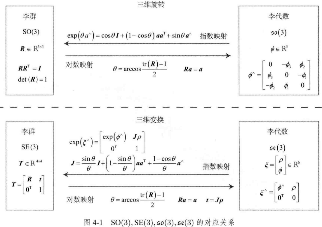
  Thanks to $J$ can be given by$\varphi$ is obtained, so here$\rho$ can also be solved from this linear equation. Now, we have clarified the definitions of Lie groups and Lie algebras and their mutual transformation relations, as shown in the figure below:

4.3 Lie algebraic derivation and disturbance model

4.2.1 BCH formula and approximate form

  One of the main motivations for using Lie algebras is optimization, where derivatives are very necessary information. Let's consider a problem. Although we have cleared $SO\left(3\right)$ sumSE$The\; relation\; between\; Lie\; group\; and\; Lie\; algebra\; on\; SE\left(3\right)$ , but when on$When\; two\; matrices\; are\; multiplied\; in\; SO\left(3\right)$ , in Lie algebra$What\; has\; changed\; on\; so\left(3\right)$ ? Conversely, whenso ( 3 ) \mathfrak{so}(3)When adding two Lie algebras on$so$$($$3$$)$$Does\; SO\left(3\right)$ correspond to the product of two matrices? If true, it is equivalent to:

         $\exp ({\varphi }_1^{\wedge })\exp \left({\varphi }_2^{\wedge }\right)=\exp (({\varphi }_1+{\varphi }_2{)}^{\wedge })?$

  如果${\varphi }_1,{\varphi }_2$为标量，那么显然该式成立；但此时我们计算的是矩阵的指数函数，而非标量的指数。换言之，我们在研究下式是否成立：

         $\ln (\exp (A)\exp (B))=A+B？$

  很遗憾，该式在矩阵时并不成立。两个李代数指数映射乘积的完整形式，由Baker-Campbell-Hausdorff公式(BCH公式)给出。由于其完整形式较复杂，我们只给出其展开式的前几项：

         $\ln (exp(A)\exp (B))=A+B+\frac{1}{2}[A,B]+\frac{1}{12}[A,[A,B]]-\frac{1}{12}[B,[A,B]]+\cdot \cdot \cdot$

  where $[]$ are the braces. The BCH formula tells us that when dealing with the product of two matrix exponents, they result in some remainder consisting of Lie brackets. In particular, consider$Lie$ algebraln ⁡ ( exp ( ϕ 1 ∧ ) exp ⁡ ( ϕ 2 ∧ ) ) ∨ , \ln(exp(\phi_1^{\land})\exp(\phi_2^{$\backslash$$land$$\}$$\ln \left(exp\right({\varphi }_1^{\wedge })\exp ({\varphi }_2^{\wedge }){)}^{\vee },$when${\varphi }_1$or ${\varphi }_2$When it is a small amount, the items above the second degree of the small amount can be ignored. At this time, BCH has a linear approximate expression:

         $\ln \left(exp\right({\varphi }_1^{\wedge })\exp ({\varphi }_2^{\wedge }){)}^{\vee }\approx \{\begin{array}{ll}{J}_l({\varphi }_2{)}^{-1}{p}_1+{\varphi }_2& 当{\varphi }_{1}for\; a\; small\; amount,\\ J_r({\varphi }_1{)}^{-1}{p}_2+{\varphi }_1& 当{\varphi }_{2}for\; a\; small\; amount\end{array}$

  Take the first approximation as an example. This formula tells us that when for a rotation matrix $R_2$(The Lie algebra is ${\varphi }_2$) is left multiplied by a small rotation matrix $R_1$(The Lie algebra is ${\varphi }_1$), it can be approximately regarded as, in the original Lie algebra ${\varphi }_2$A term J l ( ϕ 2 ) − 1 ϕ 1 is added to it . $J_l({\varphi }_2{)}^{-1}{p}_1.$Similarly, the second approximation describes the case of right multiplication by a small displacement. Therefore, under the BCH approximation, Lie algebra is divided into two types: left multiplication approximation and right multiplication approximation. When using it, we must pay attention to whether we use the left multiplication model or the right multiplication model.
  This book uses left multiplication as an example. Left multiplication BCH approximation Jacobian$J_l$In fact, it is the content of formula (4.27):

         $J_l=J=\frac{\sin \theta }{i}I+(1-\frac{\sin \theta }{\theta })a{a}^T+\frac{1-\cos \theta }{\theta }{a}^{\wedge }.$

  它的逆为

         $J_l^{-1}=\frac{\theta }{2}\cot \frac{\theta }{2}I+(1-\frac{\theta }{2}\cot \frac{\theta }{2})a{a}^T-\frac{\theta }{2}{a}^{\wedge }.$

而右乘雅可比仅需要对自变量取负号即可：

         $J_r(\varphi )=J_l(-\varphi ).$

  这样，我们就可以谈论李群乘法与李代数加法的关系了。
  为了方便读者理解，我们重新叙述BCH近似的意义。假定对某个旋转$R,$ 对应的李代数为$\varphi .$We multiply it to the left by a small rotation, denoted as$\Delta R,$ the corresponding Lie algebra is$\Delta \varphi .\_$Then, on the Lie group, the result obtained is$\Delta R\cdot R,$ and on the Lie algebra, according to the BCH approximation, is$J_l^{-1}\left(\varphi \right)D\varphi +\varphi .$Combined, it can be simply written as:

         $\exp (\Delta {\varphi }^{\wedge })\exp \left({\varphi }^{\wedge }\right)=\exp ((\varphi +J_l^{-1}\left(\varphi \right)D\varphi {)}^{\wedge }).$

  Conversely, if we perform addition on Lie algebras, let a $\varphi$ plusΔ$\Delta \varphi ,$ let a$\varphi$ plusΔ$\Delta \varphi ,$ then it can be approximated as multiplication with left and right Jacobians on Lie groups:

         $\exp ((\varphi +D\varphi {)}^{\wedge }))=\exp ((J_{l}D\varphi {)}^{\wedge })\exp ({\varphi }^{\wedge })=\exp ({\varphi }^{\wedge })\exp ((J_r\Delta \varphi {)}^{\wedge }).$

  这就为之后李代数上做微积分提供了理论基础。同样地，对于$SE(3),$也有类似的BCH近似：

         $\exp (\Delta {\xi }^{\wedge })\exp ({\xi }^{\wedge })\approx \exp (({\mathcal{J}}_l^{-1}\Delta \xi +\xi {)}^{\wedge }),$
         $\exp ({\xi }^{\wedge })\exp \left(D{\xi }^{\wedge }\right)\approx \exp (({\mathcal{J}}_r^{-1}Dx+x{)}^{\wedge }).$

  Here the form of $\mathcal{J_l} is more complex, it is a $6\times 6$ matrix. Since we did not use the Jacobian in the calculation, its actual form is omitted here.

4.3.2 Derivation of Lie algebras on SO(3)

  Let's discuss a function with a Lie algebra and the problem of derivation of the Lie algebra. The question has a strong practical background. In SLAM, we want to estimate the position and pose of a camera given by SO ( 3 ) SO(3)Rotation matrix on$SO$$($$3$$)$ or SE(3) SE(3)Described by the transformation matrix on$SE$$($$3$$)\; .$It may be advisable to set the pose of the little radish as$T.\_$It observes a world coordinate at$The\; point\; of\; p$ produces an observation data$z.$Then, from the coordinate transformation relation:

         $z=Tp+w.$

in that $w$ is random noise. Because of its existence,$It\; is\; often\; impossible\; for\; z$ to satisfy z = T pz = Tpexactly$z=Tp$ relationship. Therefore, we usually calculate the error between the ideal observation and the actual data:

         $e=z-Tp.$

  Suppose there are $N$ such landmark points and observations, so there are$N$ above formulas. Then, estimating the pose of the radish is equivalent to finding an optimal$T,$ so that the overall error is minimized:

         $\underset{T}{\min }J(T)=\sum _{i=1}^N\Vert z_i-T{p}_i{\Vert }_2^2.$

  To solve this problem, it is necessary to calculate the objective function $J$ with respect to the transformation matrixTTDerivative of$T.$We leave the specific algorithm for later. The point here is that we often construct pose-related functions and then talk about derivatives of that function with respect to pose to adjust the current estimate. **However,$SO\left(3\right),$ SE ( 3 ) SE(3)There are no well-defined additions on$SE$$($$3$$)\; ,\; they\; are\; just\; groups.$If we take$T$ is treated as an ordinary matrix to handle optimization, and it must be constrained. From the perspective of Lie algebra, since Lie algebra is composed of vectors and has good addition operations, there are two ways to use Lie algebra to solve the problem of derivation:

1. 用李代数表示姿态，然后根据李代数加法对李代数求导。
2. 对李群左乘或右乘微小扰动，然后对该扰动求导，称为左扰动和右扰动模型。

  第一种方式对应到李代数的求导模型，而第二种方式则对应到扰动模型。下面讨论下这两种思路的异同。

4.3.3 李代数求导

  首先，考虑$SO(3)$上的情况。假设我们对一个空间点$p$进行了旋转，得到了$Rp$。现在，要计算旋转之后点的坐标相对于旋转的导数，我们非正式地记为

                  $\frac{\partial (Rp)}{\partial (R)}$

由于$SO(3)$没有加法，所以该导数无法按照导数的定义进行计算。设$R$对应的李代数为$\varphi ，$我们转而计算：

                  $\frac{\partial \left(exp\right({\varphi }^{\wedge })p)}{\partial \varphi }.$

  According to the definition of derivative, we have

         $\begin{array}{rl}\frac{\partial (\exp ({\varphi }^{\wedge })p)}{\partial \varphi }& =\underset{\delta \varphi \to 0}{\lim }\frac{\exp ((\varphi +\delta \varphi {)}^{\wedge })p-\exp ({\varphi }^{\wedge })p}{\delta \varphi }\\ & \\ & =\underset{\delta \varphi \to 0}{\lim }\frac{\exp ((J_l\delta \varphi {)}^{\wedge })\exp ({\varphi }^{\wedge })p-\exp ({\varphi }^{\wedge })p}{\delta \varphi }\\ & \\ & =\underset{\delta \varphi \to 0}{\lim }\frac{(I+(J_l\delta \varphi {)}^{\wedge })\exp ({\varphi }^{\wedge })p-\exp ({\varphi }^{\wedge })p}{\delta \varphi }\\ & \\ & =\underset{\delta \varphi \to 0}{\lim }\frac{(J_l\delta \varphi {)}^{\wedge }\exp ({\varphi }^{\wedge })p}{\delta \varphi }\\ & \\ & =\underset{\delta \varphi \to 0}{\lim }\frac{-(\exp ({\varphi }^{\wedge })p{)}^{\wedge }{J}_l\delta \varphi }{\delta \varphi }=-(Rp{)}^{\wedge }{J}_l\end{array}$

  The approximation in line 2 is the BCH linear approximation, and the approximation in line 3 after Taylor expansion discarding higher-order terms (because the limit is taken, you can write an equal sign), lines 4 to 5 regard the antisymmetric symbol as the cross product, Change the number after the exchange. Thus, we derive the derivative of the rotated point with respect to the Lie algebra:

         $\frac{\partial (Rp)}{\partial \varphi }=(-Rp{)}^{\wedge }{J}_l.$

  However, since there are still complex forms of $J_l,$ we do not wish to compute it. The perturbation model described below provides a simpler way to calculate the derivative.

4.3.4 Disturbance model (left multiplication)

  Another way of derivation is to $R$ performs a disturbance$\Delta R$ , look at the rate of change of the result relative to the disturbance. This disturbance can be multiplied on the left or on the right, and the final result will be slightly different. Let's take the left disturbance as an example. Let the left disturbance$\Delta R$ corresponds to the Lie algebra$\phi$$\phi .$Then, for$\phi$ derivative, namely

         $\frac{\partial (Rp)}{\partial \phi }=\underset{\phi \to 0}{\lim }\frac{exp(f^{\wedge })exp({\varphi }^{\wedge })p-exp({\varphi }^{\wedge })p}{Phi}.$

  The derivative of this formula is simpler than the above:

         $\begin{array}{rl}\frac{\partial (Rp)}{\partial \phi }& =\underset{\phi \to 0}{\lim }\frac{\exp (f^{\wedge })\exp ({\varphi }^{\wedge })p-\exp ({\varphi }^{\wedge })p}{Phi}\\ & \\ & =\underset{\phi \to 0}{\lim }\frac{(I+{Phi}^{\wedge })\exp \left({\varphi }^{\wedge }\right)p-\exp \left({\varphi }^{\wedge }\right)p}{Phi}\\ & \\ & =\underset{\phi \to 0}{\lim }\frac{{Phi}^{\wedge }Rp}{Phi}=\underset{\phi \to 0}{\lim }\frac{-(Rp{)}^{\wedge }\phi }{Phi}=-(Rp{)}^{\wedge }.\end{array}$

  It can be seen that compared with directly deriving Lie algebras, a Jacobian $J_l$calculation. This makes the perturbation model more practical. Readers must understand the derivative operation here, which is of great significance in pose estimation.

4.3.5 Derivation of Lie algebras on SE(3)

  Finally, we give $The\; perturbation\; model\; on\; SE\left(3\right)$ and the derivation on direct Lie algebra are not introduced anymore. Assume that a certain spatial point$p$ undergoes a transformation$T$ (corresponding to Lie algebra is$\xi$ ), get$Tp$ . Now, to$T$ is left multiplied by a disturbance$\Delta T=\exp \left(\delta {\xi }^{\wedge }\right),$we set the Lie algebra of the disturbance term as$dx=[dr,d\varphi {]}^T,$then:

         $\begin{array}{rl}\frac{\partial (Tp)}{\partial \delta \xi }& =\underset{\delta \xi \to 0}{\lim }\frac{\exp (\delta {\xi }^{\wedge })\exp ({\xi }^{\wedge })p-\exp ({\xi }^{\wedge })p}{dx}\\ & \\ & =\underset{\delta \xi \to 0}{\lim }\frac{(I+d{x}^{\wedge })\exp \left({\xi }^{\wedge }\right)p-\exp \left({\xi }^{\wedge }\right)p}{dx}\\ & \\ & =\underset{\delta \xi \to 0}{\lim }\frac{d{x}^{\wedge }\exp \left({\xi }^{\wedge }\right)p}{dx}\\ & \\ & =\underset{\phi \to 0}{\lim }\frac{\left[\begin{array}{cc}d{\varphi }^{\wedge }& dr\\ & \\ 0^T& 0\end{array}\right]\left[\begin{array}{c}Rp+t\\ \\ 1\end{array}\right]}{dx}\\ & \\ & =\underset{\phi \to 0}{\lim }\frac{\left[\begin{array}{c}d{\varphi }^{\wedge }(Rp+t)+dr\\ \\ 0^T\end{array}\right]}{[dr,d\varphi {]}^T}=\left[\begin{array}{cc}I& -(Rp+t{)}^{\wedge }\\ & \\ 0^T& 0^T\end{array}\right]\stackrel{def}{=}(Tp{)}^{⨀}.\end{array}$

  We define the final result as an operator ${}^{⨀}$ , which transforms a space point of homogeneous coordinates into a$4\times 6$ matrix. What needs to be explained in this formula is the order of matrix derivation, assuming$a,b,x,Both\; y$ are column vectors, so in our writing method, there are the following rules:

         $\frac{d\left[\begin{array}{c}\\ \\ a\\ \\ b\\ \end{array}\right]}{d\left[\begin{array}{c}\\ \\ x\\ \\ y\\ \end{array}\right]}=\left(\frac{d[a,b{]}^T}{d\left[\begin{array}{c}\\ \\ x\\ \\ y\\ \end{array}\right]}\right)={\left[\begin{array}{cc}\frac{d}{dx}& \frac{db}{dx}\\ & \\ \frac{d}{dy}& \frac{db}{dy}\end{array}\right]}^T=\left[\begin{array}{cc}\frac{d}{dx}& \frac{d}{dy}\\ & \\ \frac{db}{dx}& \frac{db}{dy}\end{array}\right]$

  So far, we have introduced Lie groups and differentiation operations on Lie algebras. In the following chapters, we will apply this knowledge to solve practical problems. Some important mathematical properties of Lie groups and Lie algebras are left as exercises for the reader.

4.4 Practice: Sophus

4.4.1 Basic usage of Sophus

  Now that we've covered the introductory knowledge of Lie algebra, it's time to walk through and solidify what you've learned with practice. Let's discuss how to manipulate Lie algebras in programs. In Lecture 3, we saw that Eigen provides a geometry module, but no support for Lie algebras. A good Lie algebra library is the Sophus library maintained by Strasdat. The Sophus library supports SO ( 3 ) SO(3) which is mainly discussed in this chapter$SO\left(3\right)$ Sum$SE\left(3\right),$ in addition, also contains two-dimensional motion$SO(2),SE\left(2\right)$ and the content of similar transformation Sim ( 3 ). It is directly developed on the basis of Eigen, we don't need to install additional dependencies. Early versions of Sophus only provided double-precision Lie groups/Lie algebra classes. Subsequent versions changed to template classes. Lie groups/Lie algebras of different precision can be used in Sophus of the template class, but at the same time, it increases the difficulty of use. In this book, we usewith templates.
  For details, seeSO(3) SO(3)slambook/ch4/useSophus.cppto demonstrate the Sophus library$SO\left(3\right)$ sumSE$SE\left(3\right)$ operation:
  the operation result is as follows:

  the above program demonstrates the content of two parts. The first half introducesSO ( 3 ) SO(3)Operations on$SO$$($$3$$)$$SE\left(3\right).$We demonstrate how to construct$SO(3),SE\left(3\right)$ objects, how to perform exponential and logarithmic mapping on them, and how to update the Lie group elements when the updating amount is known. When you understand the content of this lecture, then this program should not be difficult for you. In order to compile, you need to add the following lines of code to CMakeLists.txt:

find_package( Sophus REQUIRED)
include_directories( ${
    
    Sophus_INCLUDE_DIRS})

add_executable( useSophus useSophus.cpp)

  The find_package command is an instruction provided by cmake to find the header files and library files of a certain library. If cmake can find it, it will provide the variable for the directory where the header and library files are located. In the case of Sophus, it is Sophus_INCLUDE_DIRS. Template-based Sophus libraries, like Eigen, contain only header files and no source files. According to them, we can import the Sophus library into our own cmake project.

4.4.2 Example: Evaluating Trajectory Errors

  In practical engineering, we often need to evaluate the difference between the estimated trajectory of an algorithm and the real trajectory to evaluate the accuracy of the algorithm. The true trajectory is often obtained by some higher-precision system, while the estimated trajectory is calculated by the algorithm to be evaluated. In the third lecture, we demonstrated how to display a track stored in a file. In this section, we consider how to calculate the error of two tracks. Consider an estimated trajectory $T_{it\text{'}sti,}$and the real trajectory $T_{gt,i},$ of which$i=1,\cdot \cdot \cdot ,N,$ then we can define some error metrics to describe the difference between them.
  There are many kinds of error indicators, the common one isabsolute trajectory error (Absolute Trajectory Error, ATE),in the form of:

         $AT{E}_{all}=\sqrt{\frac{1}{N}\sum _{i=1}^N\Vert \log (T_{gt,i}^{-1}{T}_{it\text{'}sti,}{)}^{\vee }{\Vert }_2^2},$

This is actually the Root-Mean-Squared Error (RMSE) of the Lie algebra for each pose . This error can characterize the rotational and translational errors of the two trajectories. At the same time, some literature only considers the translation error, so that the absolute translation error (Avergae Translational Error) can be defined:

         $AT{E}_{trans}=\sqrt{\frac{1}{N}\sum _{i=1}^N\Vert trans(T_{gt,i}^{-1}{T}_{it\text{'}sti,}){\Vert }_2^2},$

Among them, trans means to take the translation part of the variable inside the brackets. Because from the perspective of the entire trajectory, after an error occurs in the rotation, the subsequent trajectory will also have an error in translation, so both indicators are applicable in practice.
  In addition to this, relative errors can also be defined. For example, consider $i$时刻到$i+The\; motion\; at\; time\; \Delta t$ , then the relative pose error can be defined as$:$

         $RP{E}_{all}=\sqrt{\frac{1}{N-\Delta t}\sum _{i=1}^{N-\Delta t}\Vert \log ((T_{gt,i}^{-1}{T}_{gt,i+\Delta t}{)}^{-1}(T_{isti,i}^{-1}{T}_{esti,i+\Delta }){)}^{\vee }{\Vert }_2^2},$

Similarly, only the translation part can be taken:

         $RP{E}_{trans}=\sqrt{\frac{1}{N-\Delta t}\sum _{i=1}^{N-\Delta t}\Vert trans((T_{gt,i}^{-1}{T}_{gt,i+\Delta t}{)}^{-1}(T_{isti,i}^{-1}{T}_{esti,i+\Delta })){\Vert }_2^2},$

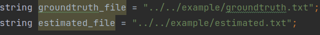
  Using the Sophus library, it is easy to implement this part of the calculation. Next, we demonstrate the calculation of the absolute trajectory error. In this example, we have two trajectories, groundtruth.txt and estimated.txt, the following code will read these two trajectories, calculate the error, and then display it in the 3D window. For the sake of brevity, the code for drawing the trajectory is omitted. We have done something similar in Lecture 3.
  Code See slambook/ch4/example/trajectoryError.cpp
  The process of making the code run successfully is also an unusual twists and turns, divided into three steps:

1. First of all, the fmt library is missing because the new version of Sophus not only needs Pangolin, but also needs to install fmt, so just install it.
2. After installation and running, he will still report an error. fmt/core.h:1711:3: error: static assertion failed: Cannot format an argument.Baidu said that it is a version problem. It is recommended to use fmt 8.1.1 . Okay, the next version of fmt 8.1.1 does not need to delete the previous version, just repeat the previous steps
3. After installation, remember to add the following two sentences in CMakeLists.txt, let cmake include this library, so that the program can run

find_package(FMT REQUIRED) 
target_link_libraries(trajectoryError fmt::fmt)

4. Then you will find that the file address is wrong, and the directory of the two txt files cannot be found. Then you need to modify the directory of the file. It
   
   took me almost an hour to run this code~!!
   The result is as follows:
   
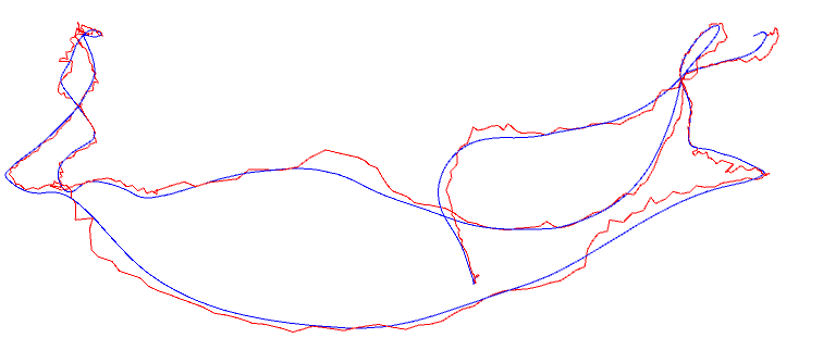
     the output of the program is 2.20728. Of course, the rotation part can also be removed, and only the error of the translation part can be calculated. As far as this example is concerned, we have actually helped readers do some preprocessing tasks, including time alignment of trajectories and external parameter estimation. These contents have not been mentioned yet, but will be mentioned in future studies.

4.5 * Groups of similar transformations and Lie algebras

Finally, we would like to mention the similarity group S im ( 3 ) Sim(3)   used in monocular vision$Sim\left(3\right)$ , and the corresponding Lie algebra$sim\left(3\right).$
  We have already introduced monocular scale uncertainty. If using SE ( 3 ) SE(3)in monocular SLAM$SE\left(3\right)$ represents the pose, then due to scale uncertainty and scale drift, the scale of the entire SLAM process will change, which is inSE ( 3 ) SE (3)It is not reflected in$SE$$($$3$$)\; .$Therefore, in the monocular case, we generally express the scale factor explicitly. In mathematical language, for a point$p$ , in the camera coordinate system, it needs to undergo asimilar transformationinstead of Euclidean transformation:

         $p^{{}^{\prime }}=\left[\begin{array}{cc}sR& t\\ & \\ 0^T& 1\end{array}\right]p=sRp+t.$

In the similarity transformation, for us the scale $s$ is expressed. It also acts onppAbove the 3 coordinates of$p$$p$ is scaled once. with$SO\left(3\right)andSE\left(3\right)$ are similar, and the similar transformation also forms a group for matrix multiplication, which is called the similar transformation group Sim(3):

         $Sim(3)=\left\{\begin{array}{c}S=\left[\begin{array}{cc}sR& t\\ & \\ 0^T& 1\end{array}\right]\in R^{4\times 4}\end{array}\right\}$

  Similarly, Sim(3) also has corresponding Lie algebras, exponential maps, logarithmic maps, etc. Lie algebra $The\; sim\left(3\right)$ element is a 7-dimensional vector$z$ . Its first 6 dimensions are related to$se\left(3\right)$ is the same, but there is an extra term$s$ .

         $\mathfrak{sim}(3)=\left\{\begin{array}{c}\zeta |\zeta =\left[\begin{array}{c}r\\ \\ \varphi \\ \\ \end{array}\right]\in R^7,g^{\wedge }=\left[\begin{array}{cc}\sigma I+{\varphi }^{\wedge }& r\\ & \\ 0^T& 0\end{array}\right]\in R^{4\times 4}\end{array}\right\}$

  It is better than $se\left(3\right)$ has one more term$\sigma$ . Associate Sim(3) with$sim\left(3\right)$ is still exponential mapping and logarithmic mapping. Index maps to

         $\exp (g^{\wedge })=\left[\begin{array}{cc}{e}^p\exp \left({\varphi }^{\wedge }\right)& J_{s}r\\ & \\ 0^T& 1\end{array}\right].$

  Among them, $J_s$in the form of

         $\begin{array}{rl}{J}_s& =\frac{e^p-1}{p}I+\frac{in{e}^p\sin i+(1-e^p\cos i)}{p^2+i^2}{a}^{\wedge }\\ & +\left(\frac{e^p-1}{p}-\frac{(e^p\cos i-1)p+\left(e^p\sin i\right)}{p^2+i^2}\right)a^{\wedge }{a}^{\wedge }.\end{array}$

  Through exponential mapping, we can find the relationship between Lie algebras and Lie groups. For Lie algebra $\zeta ,$ and its correspondence with Lie groups is

         $s=e^s,R=\exp ({\varphi }^{\wedge }),t=J_{s}r.$

  The rotating part is consistent with SO(3). The translation part, in $In\; se(3),$ it is necessary to multiply a Jacobian$J,$ and the Jacobian of the similarity transformation is more complex. For the scale factor, one can see ssin the Lie group$s$ is σ \sigmain Lie algebraExponential function of$\sigma \; .$
  The BCH approximation of Sim(3) is similar to SE(3). we can discuss a point$p$ undergoes similarity transformation$Sp$ , relative toSSDerivative of$S.$Similarly, there are two ways, the differential model and the disturbance model, and the disturbance model is relatively simple. We omit the derivation process and directly give the results of the perturbation model. LetS p Sp SpA small disturbance on the left side$of\; Sp$$\exp \left(g^{\wedge }\right),$and findS p SpThe derivative of$Sp\; with\; respect\; to\; the\; disturbance.$Because$Sp$ is a 4-dimensional homogeneous coordinate,$\zeta$ is a 7-dimensional vector, so the derivative should be$4\times$Jacobian of$7\; .$For convenience, denoteS p SpThe first 3-dimensional composition vector of$Sp$$q,$ then:

         $\frac{\partial Sp}{\partial \zeta }=\left[\begin{array}{ccc}I& -q^{\wedge }& q\\ & & \\ 0^T& 0^T& 0\end{array}\right]$

4.6 Summary

  This lecture introduces Lie groups SO(3) and SE(3), and their corresponding Lie algebras $so\left(3\right)$ and$se\left(3\right).$We introduced the expression and transformation of the pose on them, and then through the linear approximation of BCH, the pose can be perturbed and derived. This lays a theoretical foundation for explaining the optimization of the pose later, because we need to frequently adjust the estimated value of a certain pose to reduce its corresponding error. Only after you have figured out how to adjust and update the pose can you move on.
  It is worth mentioning that, in addition to Lie algebra, rotation can also be represented by quaternion, Euler angle, etc., but the subsequent processing is more troublesome. In practical applications, SO(3) plus translation can also be used instead of SE(3), thereby avoiding some Jacobian calculations.