written in front
Huang Ningran, after reading the algorithm you read, it is a flaw if you are not good at mathematics.
Source of problem:
An***** xue100: https://bbs.csdn.net/topics/********?spm=1001.2014.3001.**77
(1) The camera is placed on the ground, far from the ceiling The height is always the same. Take a picture at a certain position, then move the camera a certain distance, rotate a certain angle, and then take another picture. Are the feature points on these two pictures consistent in gradient value and gradient direction?
(2) opencv does not provide features of a single point, unless you do it yourself.
1. References town building
[0] David G.Lowe, distinctive image features from scale invariant keypoints.pdf
[1] Zheng Hao, Research on Image Matching Algorithm Based on Improved SIFT Algorithm
[2] Xu Xinjian, FPGA Accelerated Implementation of SIFT Image Matching Algorithm
[3] Derle3er, Python implements the SIFT algorithm, with detailed formula derivation and code
(https://blog.csdn.net/sakurakawa/article/details/120833167?spm=1001.2014.3001.5502)
[4] Brook_icv, detailed explanation of SIFT features (https://www .cnblogs.com/wangguchangqing/p/4853263.html)
[5] zddhub, SIFT algorithm detailed explanation (https://blog.csdn.net/zddblog/article/details/7521424)
[6] rmislam, SIFT source code, (https ://github.com/rmislam/PythonSIFT)
[7] Liang Shuang, Research on Image Matching Method Based on SIFT Operator
[8] Qiu Xiaodong, Realization and Optimization of SIFT Image Matching System Based on FPGA
[9] Feng Shaofeng, in opencv Match and KnnMatch return value explanation (https://blog.csdn.net/weixin_44072651/article/details/89262277)
2. Overview of SIFT algorithm
The full name of SIFT is Scale Invariant Feature Transform, which is translated as scale invariant feature transformation. It is mainly used to obtain the features of the image. It has scale invariance, rotation invariance, and brightness invariance [1].
Generally, finding the features of an image is to find the feature points in the image, and the same is true for the SIFT algorithm, whose main task is to find the feature points in the image. The feature points are generally to find the extreme points of the image in some aspects, such as the extreme points on the pixel value. To find extreme points, generally compare the difference, for example, find the edge of the image through the difference.
A good feature point finding algorithm should not change with the scale change of the image (such as image zoom in and out), rotation change, and brightness change. For example, after algorithm processing, a certain image position is an extreme point when the image is enlarged by 1:1, and it is also an extreme point when the image is enlarged by 1:0.5, so the extreme point is more credible.
In general, the SIFT algorithm includes the following steps: constructing scale space, finding extreme points, calculating the direction of extreme points, and generating descriptions of extreme points [2].
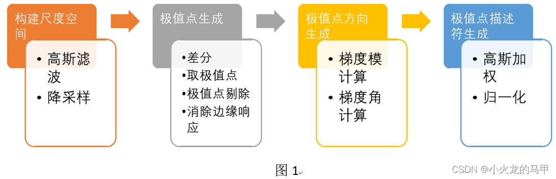
(1) To construct the scale space, that is, to obtain the image to transform the image at different scales (such as 1:1, 1:0.5, etc.), and to obtain it in combination with Gaussian filtering and down-sampling; (2) To find extreme points, that is, to
synthesize Images at various scales (difference images), looking for extreme positions, that is, not only finding extreme points on a certain image, but looking for extreme points on multiple images of different scales, the purpose is to extract multiple scales common features below. Because features that exist simultaneously in multiple scales have different degrees of scale invariance. If a feature spans more scales, its invariance will be better [2].
(3) Finding the extreme point is only to obtain the position and scale information. In order to meet the rotation invariance, it also needs to cover the direction information of the extreme point, such as calculating the gradient direction to obtain the direction of the extreme point; (4) When generating the extreme
point description, on the one hand, the amplitude information of the extreme point information can be normalized to ensure the brightness invariance. Similarly, the extreme point direction information " "Normalization" (such as rotating the image by a certain angle and returning the direction of the extreme point to zero) can guarantee rotation invariance (personal understanding).
In the following, we start to analyze these aspects in detail.
3. construct scale space
3.1 Brief introduction
Scale space construction is mainly to downsample and Gaussian filter the image. Directly above the picture [2].
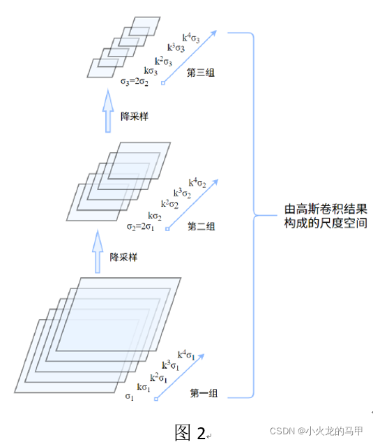
Constructing the scale space is actually obtaining the image Gaussian pyramid. As shown in Figure 2, it is assumed that the first group is the size of the original image, the second group is the 1/2 size downsampling of the first group, and the third group continues to 1/2 downsampling. If only the downsampling operation is performed, it may be slightly rough. Here, the Gaussian scale space is introduced again, that is, for each set of input images, the images are Gaussian filtered using different standard deviations σ. An important parameter of Gaussian filtering is the standard deviation σ, which represents the scale factor. The larger the σ is, the more blurred it is, and the more global the image can be seen.
Combined with Figure 2, first look at the first group, using σ 1 , K σ 1 , K 2 σ 1 … σ_1 , Kσ_1 , K^2 σ_1…p1、K p1、K2 p1... gaussian filtering the input image for a range of standard deviations. This series of standard deviations (scales) constitutes the different scales s in the group, which is called a layer, and this group is also called an octave, and the images at each scale in each group have the same size. The second group of images is first down-sampled from the first group of images, and then Gaussian filtering is also performed on the images using a series of standard deviations to form the scale space of the second group of images.
To ensure continuity, the initial standard deviation of the second group is twice the initial standard deviation of the first group.
Assuming that each group performs S-layer scale filtering, the scale factor coefficient between adjacent layers of each group is taken:
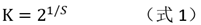
For the first group, the standard deviation of each s layer is:
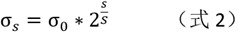
for the oth group, the sth layer, the standard deviation For:
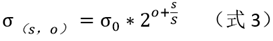
hereσ 0 σ_0p0is the initial standard deviation (initial scale factor).
For the first group, when s=S+1, σ s = σ 0 ∗ 2 σ_s=σ_0*2ps=p0∗2 , which is exactly the initial standard deviation of the next group.
Therefore, the Gaussian filter result image of layer s=S+1 is downsampled by 1/2 as the input image of the second group.
Note:
(1) The nature of Gaussian filtering, sequentially performσ 1 , σ 2 σ_1 , σ_2p1、p2Gaussian filtering twice, which is equivalent to performing a σ 3 σ_3 on the image oncep3Gaussian filtering with the following constraints: σ 3 2 = σ 1 2 + σ 2 2 σ_3^2= σ_1^2+σ_2^2p32=p12+p22
Therefore, for each group, the Gaussian filtering result of the next layer can be performed on the previous Gaussian filtering result, and only the middle standard deviation σ 2 σ_2 is requiredp2That's it.
(2) For each group, when calculating the Gaussian filter of the group of images, according to (Formula 3), it can be known that σ is related to octave. But in the code of rmislam [6], the value of σ of this group is only related to layer s. Why? Is it because: for each group, the input image of this group has been downsampled by 1/2 on the basis of the previous group, covering 2 o 2^o2The information of o , ie (Equation 3) refers to the scale factor relative to the original input image, not relative to the scale factor under the set of octaves. I don't know if this understanding is correct?
(3) For the input image, if it is taken by a camera, the camera has generally been blurred by σ=0.5, which needs to be considered for conversion in subsequent calculations.
(4) Selection of parameters for constructing scale space.
According to literature [7], DGLowe suggested σ=1.6, S=3. Determination of the number o of Gaussian pyramid groups:

M and N are the width and height of the image.
In addition, the subsequent calculation of the extreme point of the difference layer is to compare the pixel values of the difference layer with the upper layer and the lower layer at the same time. In order to obtain S layer results, S+2 difference layers are required, and S+2+1 Gaussian layers are required. See the description below for details. Therefore, the scale of the penultimate third layer (s=S+1) in the group is exactly the initial scale of the next group.
3.2 python code
#coding=utf8
import numpy as np
from PIL import Image
import matplotlib.pyplot as plt
import matplotlib.cm as cm
import math
import cv2
import os,sys
import scipy.ndimage
import time
import scipy
from numpy.linalg import det, lstsq, norm
from functools import cmp_to_key
(1) Define the CSift class for parameter passing
###################################################### 1. 定义SIFT类 ####################################################
class  CSift:
	def __init__(self,num_octave,num_scale,sigma):
		self.sigma = sigma	#初始尺度因子
		self.num_scale = num_scale #层数
		self.num_octave = 3 #组数,后续重新计算
		self.contrast_t = 0.04#弱响应阈值
		self.eigenvalue_r = 10#hessian矩阵特征值的比值阈值
		self.scale_factor = 1.5#求取方位信息时的尺度系数
		self.radius_factor = 3#3被采样率
		self.num_bins = 36 #计算极值点方向时的方位个数
		self.peak_ratio = 0.8 #求取方位信息时,辅方向的幅度系数
(2) Preprocessing pictures
###################################################### 2. 构建尺度空间 ####################################################
def pre_treat_img(img_src,sigma,sigma_camera=0.5):
	sigma_mid = np.sqrt(sigma**2 - (2*sigma_camera)**2)#因为接下来会将图像尺寸放大2倍处理,所以sigma_camera值翻倍
	img = img_src.copy()
	img = cv2.resize(img,(img.shape[1]*2,img.shape[0]*2),interpolation=cv2.INTER_LINEAR)#注意dstSize的格式,行、列对应高、宽
	img = cv2.GaussianBlur(img,(0,0),sigmaX=sigma_mid,sigmaY=sigma_mid)
	return img
It can be seen that the img returned here is the Gaussian filtering result of σ=sigma=1.6
(3) Calculate the number of Gaussian pyramid groups
def get_numOfOctave(img):
	num = round (np.log(min(img.shape[0],img.shape[1]))/np.log(2) )-1
	return num
(4) Build a Gaussian pyramid
def construct_gaussian_pyramid(img_src,sift:CSift):
	pyr=[]
	img_base = img_src.copy()
	for i in range(sift.num_octave):#共计构建octave组
		octave = construct_octave(img_base,sift.num_scale,sift.sigma) #构建每一个octave组
		pyr.append(octave)
		img_base = octave[-3]#倒数第三层的尺度与下一组的初始尺度相同,对该层进行降采样,作为下一组的图像输入
		img_base = cv2.resize(img_base,(int(img_base.shape[1]/2),int(img_base.shape[0]/2)),interpolation=cv2.INTER_NEAREST)
	return pyr
build each group
def construct_octave(img_src,s,sigma):
	octave = []
	octave.append(img_src) #输入的图像已经进行过GaussianBlur了
	k = 2**(1/s)
	for i in range(1,s+3):#为得到S层个极值结果,需要构建S+3个高斯层
		img = octave[-1].copy()
		cur_sigma = k**i*sigma
		pre_sigma = k**(i-1)*sigma
		mid_sigma = np.sqrt(cur_sigma**2 - pre_sigma**2)
		cur_img = cv2.GaussianBlur(img,(0,0),sigmaX=mid_sigma,sigmaY=mid_sigma)
		octave.append(cur_img)
	return octave
4. Find the extreme point (key point) position
4.1 Difference of Gaussian layer DoG[2]
To find extreme points, it is generally found on the difference result, focusing on the local sudden changes in the image, such as points, lines, edges, etc. The SIFT algorithm detects the position of the extreme point from the Gaussian-Laplace LoG result of the image, but in order to reduce the amount of calculation, DoG is used instead, that is, for each group of Gaussian layers in Figure 2, differential processing is performed to obtain DoG, such as image 3.

4.2 Find the initial extreme point
For each layer (s) DOG under each group (octave) in Figure 3, find the extreme points, as shown in Figure 4. For the x position in Figure 4, in addition to comparing the 3*3 neighborhood of the current layer, the upper and lower neighborhoods are also compared, that is, a total of 26 pixel points are compared. Therefore, the position of the qualified extreme point should include group information octave, layer information scale, and XY information.
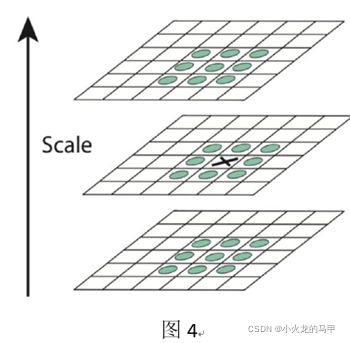
Therefore, in order to obtain the results of the extreme points of the S layer, it is necessary to construct S+2 DoG layers, and it is necessary to construct S+3 Gaussian layers.
Note:
When looking for preliminary extreme points on DoG, the extreme points need to be greater than a certain threshold (contrast threshold) to be recognized. According to the literature [8], "the first step of screening for extreme points is to eliminate those points whose DoG image is too small, and these points are susceptible to noise interference and become unstable due to the small response", assuming that the gray value of the image Between [0,1], literature [8] takes the threshold as 0.03. Derle3er [3] takes the threshold value as 0.04, and calculates the final threshold value (original image pixel value ranges from 0 to 255) through the following formula: threshold =
floor(0.5 * contrast_threshold / num_intervals * 255)
where num_intervals is the decomposition scale S, This is mentioned in Equation (2-11) in literature [1]. Why it is multiplied by 0.5 is unknown.
In addition, after the next interpolation to obtain precise positioning, weak gray values will be eliminated again.
4.3 Interpolation to obtain precise extreme point position
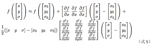
After the initial extreme point is found, it needs to interpolate to get the precise position. Because the extremum point is found in the group, the interpolation needs to use layer σ, and x, y information. Think of the pixel value as a function f(x,y, σ) of these 3 variables, and use Taylor expansion to expand f to 2 times at (x0, y0, σ0), as shown in [3].
Calculation of partial derivatives of each order (h=1):
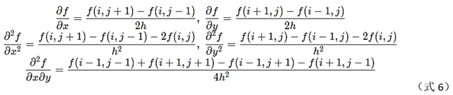
Huang Ningran, bad at mathematics, really flawed. The multivariate Taylor expansion will not be adjusted at all, and will only force the entire unary. See literature [3] for details.
Write the expression of f above as a matrix [4].
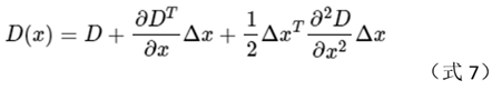
Here, I personally think that using ∆x in [4] is more appropriate than using X in other documents.
Calculate the derivative of formula (7), and set the equation to 0, the obtained value is the offset of the extreme point position, how to deduce it, I don’t know.
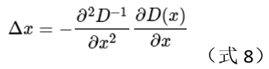
The value of f at the corresponding extreme point
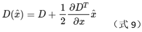
is , then the precise position of the extreme point is:
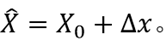
Note:
When interpolating the extreme point, if each dimension of ∆x (ie x, y, σ) is found to be less than 0.5, it is considered The interpolation is successful; if any dimension exceeds 0.5, it is considered that the position of the real extreme point is closer to other adjacent points, and X 0 X_0 needs to be updatedX0The position is re-interpolated. The number of attempts is set to 5, and if the obtained position has exceeded the image boundary, it is directly considered that the interpolation fails [2].
4.4 Elimination of edge responses [1]
Some of the extreme points obtained as above are the edges of the image, while the SIFT algorithm pays more attention to the corner-shaped feature points. Therefore, the edge feature points need to be removed.
Use the Hessian matrix to eliminate edge response points.

Among them, Dxx, Dxy, Dyx, and Dyy are the partial derivatives of the DoG scale space image in the x-axis and y-axis directions, respectively.
The basis of the idea of elimination: the H matrix at the edge has a large and small distribution of eigenvalues [2].
Let the trace and determinant of this matrix be Tr and Det respectively. Assuming that the two eigenvalues of H are α and β respectively, then there are:
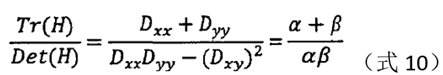
assuming that the eigenvalue of α is larger, and β is the smaller eigenvalue, let α=r*β,
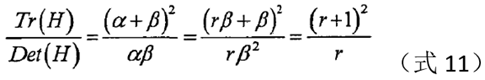
when the right side of the equation is larger, the two characteristics The greater the difference in value, that is, the gradient value in one direction is larger, while the gradient value in another direction is smaller, which is the characteristic of the edge, so it can be deleted. For the extreme points satisfying the following formula (12), they should be kept, otherwise, they should be eliminated.
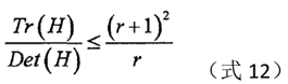
In Lowe's paper, r is taken as 10.
Note: I don't know how to derive the formulas in this section, I am not good at mathematics.
4.5 python code
(1) Build a Gaussian difference layer
###################################################### 3. 寻找初始极值点 ##################################################
def construct_DOG(pyr):
	dog_pyr=[]
	for i in range(len(pyr)):#对于每一组高斯层
		octave = pyr[i] #获取当前组
		dog=[]
		for j in range(len(octave)-1):#对于当前层
			diff = octave[j+1]-octave[j]
			dog.append(diff)
		dog_pyr.append(dog)
	return dog_pyr
(2) Obtain key points
def get_keypoints(gau_pyr,dog_pyr,sift:CSift):
	key_points = []
	threshold = np.floor(0.5 * sift.contrast_t / sift.num_scale * 255) #原始图像灰度范围[0,255]
	for octave_index in range(len(dog_pyr)):#遍历每一个DoG组
		octave = dog_pyr[octave_index]#获取当前组下高斯差分层list
		for s in range(1,len(octave)-1):#遍历每一层(第1层到倒数第2层)
			bot_img,mid_img,top_img = octave[s-1],octave[s],octave[s+1] #获取3层图像数据
			board_width = 5
			x_st ,y_st= board_width,board_width
			x_ed ,y_ed = bot_img.shape[0]-board_width,bot_img.shape[1]-board_width
			for i in range(x_st,x_ed):#遍历中间层图像的所有x
				for j in range(y_st,y_ed):#遍历中间层图像的所有y
					flag = is_extreme(bot_img[i-1:i+2,j-1:j+2],mid_img[i-1:i+2,j-1:j+2],top_img[i-1:i+2,j-1:j+2],threshold)#初始判断是否为极值
					if flag:#若初始判断为极值,则尝试拟合获取精确极值位置
						reu = try_fit_extreme(octave,s,i,j,board_width,octave_index,sift)
						if reu is not None:#若插值成功,则求取方向信息,
							kp,stemp = reu
							kp_orientation =  compute_orientation(kp,octave_index,gau_pyr[octave_index][stemp],sift)
							for k in kp_orientation:#将带方向信息的关键点保存
								key_points.append(k)
	return key_points
Note that after obtaining the key points here, the orientation of the key points will be calculated, which will be introduced in the next section.
def is_extreme(bot,mid,top,thr):
	c = mid[1][1]
	temp = np.concatenate([bot,mid,top],axis=0)
	if c>thr:
		index1 = temp>c
		flag1 = len(np.where(index1 == True)[0]) > 0
		return not flag1
	elif c<-thr:
		index2 = temp<c
		flag2 = len(np.where(index2 == True)[0]) > 0
		return not flag2
	return False

def try_fit_extreme(octave,s,i,j,board_width,octave_index,sift:CSift):
	flag = False
	# 1. 尝试拟合极值点位置
	for n in range(5):# 共计尝试5次
		bot_img, mid_img, top_img = octave[s - 1], octave[s], octave[s + 1]
		g,h,offset = fit_extreme(bot_img[i - 1:i + 2, j - 1:j + 2], mid_img[i - 1:i + 2, j - 1:j + 2],top_img[i - 1:i + 2, j - 1:j + 2])
		if(np.max(abs(offset))<0.5):#若offset的3个维度均小于0.5,则成功跳出
			flag = True
			break
		s,i,j=round(s+offset[2]),round(i+offset[1]),round(j+offset[0])#否则,更新3个维度的值,重新尝试拟合
		if i<board_width or i>bot_img.shape[0]-board_width or j<board_width or j>bot_img.shape[1]-board_width or s<1 or s>len(octave)-2:#若超出边界,直接退出
			break
	if not flag:
		return None
	# 2. 拟合成功,计算极值
	ex_value = mid_img[i,j]/255+0.5*np.dot(g, offset)#求取经插值后的极值
	if np.abs(ex_value)*sift.num_scale<sift.contrast_t: #再次进行弱响应剔除
		return None
	# 3. 消除边缘响应
	hxy=h[0:2,0:2] #获取关于x、y的hessian矩阵
	trace_h = np.trace(hxy) #求取矩阵的迹
	det_h = det(hxy) #求取矩阵的行列式
	# 若hessian矩阵的特征值满足条件(认为不是边缘)
	if det_h>0 and (trace_h**2/det_h)<((sift.eigenvalue_r+1)**2/sift.eigenvalue_r):
		kp = cv2.KeyPoint()
		kp.response = abs(ex_value)#保存响应值
		i,j = (i+offset[1]),(j+offset[0])#更新精确x、y位置
		kp.pt =  j/bot_img.shape[1],i/bot_img.shape[0] #这里保存坐标的百分比位置,免去后续在不同octave上的转换
		kp.size = sift.sigma*(2**( (s+offset[2])/sift.num_scale) )* 2**(octave_index)# 保存sigma(o,s)
		kp.octave = octave_index + s * (2 ** 8) + int(round((offset[2] + 0.5) * 255)) * (2 ** 16)# 低8位存放octave的index,中8位存放s整数部分,剩下的高位部分存放s的小数部分
		return kp,s
	return None

def fit_extreme(bot,mid,top):#插值求极值
	arr = np.array([bot,mid,top])/255
	g = get_gradient(arr)
	h = get_hessian(arr)
	rt =   -lstsq(h, g, rcond=None)[0]#求解方程组
	return g,h,rt

def get_gradient(arr): #获取一阶梯度
	dx = (arr[1,1,2]-arr[1,1,0])/2
	dy = (arr[1,2,1] - arr[1,0,1])/2
	ds = (arr[2,1,1] - arr[0,1,1])/2
	return np.array([dx, dy, ds])
def get_hessian(arr): #获取三维hessian矩阵
	dxx = arr[1,1,2]-2*arr[1,1,1] + arr[1,1,0]
	dyy = arr[1,2,1]-2*arr[1,1,1] + arr[1,0,1]
	dss = arr[2,1,1]-2*arr[1,1,1] + arr[0,1,1]
	dxy = 0.25*( arr[1,0,0]+arr[1,2,2]-arr[1,0,2] - arr[1,2,0]  )
	dxs = 0.25*( arr[0,1,0]+arr[2,1,2] -arr[0,1,2] - arr[2,1,0])
	dys = 0.25*( arr[0,0,1]+arr[2,2,1]- arr[0,2,1] -arr[2,0,1])
	return np.array([[dxx,dxy,dxs],[dxy,dyy,dys],[dxs,dys,dss]])
5. Calculation of extremum point (key point) direction
In the previous section, extreme points were obtained by comparing pixel values at different scales, and these extreme points already have stable characteristics of scale invariance [2]. Next, the position information is obtained. When it comes to orientation, it is natural to think of gradient angle.
The central idea: by calculating the gradient modulus and gradient angle of the neighborhood around the extreme point, assign a direction to each extreme point. Why calculate the gradient corresponding to the neighborhood instead of the direct extreme point position? In order to comprehensively consider and improve robustness. Why gradient mode information? If the gradient modulus is too small, it is considered a weak response and will be rejected.
5.1 Calculation steps
The calculation of the gradient is performed on the Gaussian layer G(o,s) corresponding to the extreme point. Specific steps:
(1) Find the Gaussian layer closest to the position of the extreme point (o, s), and use the image of this layer as input (
2) In the image of this layer, select the neighbor of the position of the extreme point (x, y) area. Neighborhood radius is determined by the following formula[8]
r = 3 ∗ 1.5 ∗ σ r=3*1.5*σr=3∗1.5∗σ (Equation 13)
In the formula, 3 represents the principle of three times sampling according to the scale [3], 1.5 is the scale coefficient, and σ is the scale under (o, s) where the extreme point is located (
3) For all points in the neighborhood, Find the gradient magnitude and gradient angle.
The calculation formula of gradient mode and gradient angle:

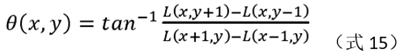
L in the formula is a Gaussian layer image.
(4) Azimuth distribution and modulus accumulation
The SIFT algorithm divides the 360° azimuth into 36 direction groups equally, and each direction group spans 10°. The gradient modulus obtained in step 3 is allocated to the 36 direction groups according to the gradient angle, and the gradient modulus in each direction group is accumulated and summed. Here, when the gradient modulus is accumulated and summed, a Gaussian weighting operation is required. Simply put, in the neighborhood, the modulus value far from the extreme point has a small contribution, and the modulus value close to the extreme point has a greater contribution.
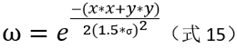
In the Gaussian weighting operation, the standard deviation of the Gaussian function is 1.5 times the current scale. Gaussian weighting coefficients:
After this step, the cumulative sum of the corresponding gradient moduli is stored in the array histogram of 36 direction groups, and the shape is like a histogram.
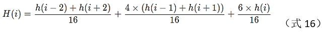
(5) Smooth filtering
Perform smooth filtering on the histogram formed in step (4), the filtering formula is as follows:
(6) Generate main direction and auxiliary direction
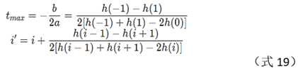
Generally speaking, for the histogram array obtained in step (5), find its maximum value The position and the direction group corresponding to the position can be used as the direction of the extremum point. In the actual operation process, in order to ensure the robustness of the algorithm, the algorithm not only retains the direction where the maximum value is located (as the main direction), but also retains the direction where the amplitude is greater than 80% of the maximum value as the auxiliary direction. Specific operation: first find the maximum value max_v of the histogram array; then, find all the local maximum points of the histogram array; for each local maximum value peak_v, if it is greater than 80%*max_v, combine its left and right two Points left_v, right_v, a total of 3 points, perform parabolic quadratic interpolation to obtain the precise position of the maximum value, and the direction obtained by converting the position is the main/auxiliary direction of the extreme point, that is, in Chapter 4, a The extreme points will correspond to multiple direction information and form multiple key points. The calculation of the precise maximum position can be based on junior high school mathematics knowledge, and the literature [3] gives a detailed description.
Assuming a parabola:
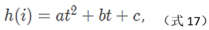
normalize each maximum value position i to 0, then the
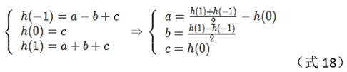
precise maximum value position is:
5.2 python code
###################################################### 4. 计算方位信息  ##################################################
def compute_orientation(kp,octave_index,img,sift:CSift):
	keypoints_with_orientations = []
	cur_scale = kp.size / (2**(octave_index)) #除去组信息o,不知为何?莫非因为输入图像img已经是进行了降采样的图像,涵盖了o的信息?
	radius = round(sift.radius_factor*sift.scale_factor*cur_scale)#求取邻域半径
	weight_sigma = -0.5 / ((sift.scale_factor*cur_scale) ** 2)#高斯加权运算系数
	raw_histogram = np.zeros(sift.num_bins)#初始化方位数组
	cx = round( kp.pt[0]*img.shape[1] )#获取极值点位置x
	cy = round( kp.pt[1]*img.shape[0] )#获取极值点位置y
	# 1.计算邻域内所有点的梯度值、梯度角,并依据梯度角将梯度值分配到相应的方向组中
	for y in range(cy-radius, cy+radius + 1): # 高,对应行
		for x in range(cx-radius, cx+radius + 1):# 宽,对应列
			if y > 0 and y < img.shape[0] - 1 and x > 0 and x < img.shape[1] - 1 :
				dx = img[y, x + 1] - img[y, x - 1]
				dy = img[y - 1, x] - img[y + 1, x]
				mag = np.sqrt(dx ** 2 + dy ** 2)#计算梯度模
				angle = np.rad2deg(np.arctan2(dy, dx))#计算梯度角
				if angle < 0:
					angle = angle + 360
				angle_index = round(angle / (360 / sift.num_bins))
				angle_index = angle_index % sift.num_bins
				weight = np.exp(weight_sigma * ((y-cy)**2 +(x-cx)**2 ))#根据x、y离中心点的位置,计算权重
				raw_histogram[angle_index] = raw_histogram[angle_index] + mag * weight#将模值分配到相应的方位组上
	# 2. 对方向组直方图进行平滑滤波
	h = raw_histogram
	ha2 = np.append(h[2:],(h[0],h[1])) # np.roll will be better
	hm2 = np.append((h[-2],h[-1]),h[:-2])
	ha1 = np.append(h[1:], h[0])
	hm1 = np.append(h[-1], h[:-1])
	smooth_histogram = ( ha2+hm2 + 4*(ha1+hm1) + 6*h)/16
	# 3. 计算极值点的主方向和辅方向
	s = smooth_histogram
	max_v = max(s)# 找最大值
	s1 = np.roll(s,1)
	s2 = np.roll(s,-1)
	index1 = s>=s1
	index2 = s>=s2
	index = np.where( np.logical_and(index1,index2)==True )[0] #找到所有极值点位置
	for i in index:
		peak_v = s[i]
		if peak_v >= sift.peak_ratio * max_v: #若大于阈值,则保留,作为主/辅方向
			left_v = s[(i-1)%sift.num_bins]
			right_v = s[(i+1)%sift.num_bins]
			index_fit= ( i+0.5*(left_v-right_v)/(left_v+right_v-2*peak_v) )%sift.num_bins#插值得到精确极值位置
			angle = 360-index_fit/sift.num_bins*360 #计算精确的方位角
			new_kp =cv2.KeyPoint(*kp.pt, kp.size, angle, kp.response, kp.octave) #在关键点中,加入方向信息
			keypoints_with_orientations.append(new_kp)
	return keypoints_with_orientations
6. Characterization of extreme points (key points)
In the previous section, the position information and orientation information of the key points have been obtained. Scale invariance of keypoints is resolved. However, rotation invariance and brightness invariance have not been resolved. Next, for each key point in the previous section, the corresponding feature descriptor is generated, and the rotation invariance and brightness invariance are guaranteed.
Similarly, in order to ensure robustness, when generating the descriptor, not only the key point information is considered, but also the neighborhood information where the key point is located, which is similar to the direction of the extreme point in the previous section. According to literature [1], feature descriptors are related to the scale of key points, and all feature descriptors are obtained on Gaussian scale images.
6.1 Neighborhood selection
According to literature [1], the original Lowe divides the neighborhood of key points into 4×4 sub-regions, and each sub-region has 8 direction information (that is, 360 degrees are divided into 8 equal parts), so each key point will eventually get 4 *4*8=128-dimensional description.
For 4×4 subregions, each subregion is a square with side length 3*σ, where σ is the scale of the current keypoint. The selection of the neighborhood is shown in Figure 5.
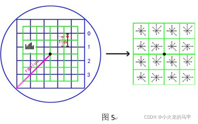
In the left part of Figure 5, the black dot in the center is the position of the key point, and the window in the green part is d×d sub-regions, where d=4, and the side length of each green box is 3*σ. The neighborhood radius is √ 2 × ( 0.5 × d × 3 × σ ) √2 × (0.5 × d × 3 × σ )√2×(0.5×d×3×σ ) , actually, it is calculated
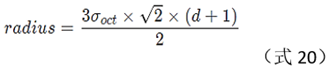
according to the following formula: Determining the descriptor is: calculating the modulus value of the 4×4 sub-regions around the key point on the 8-position group, that is, the right part of Figure 5.
6.2 Coordinate axis rotation
Each key point has direction information. After the neighborhood is determined, the entire coordinate axis is rotated so that the coordinate axis coincides with the direction of the key point. The calculation formula of the rotated coordinates is as follows:
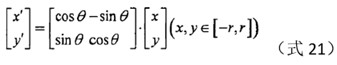
θ in the above formula is the negative number of the direction angle of the key point.
Why is it necessary to rotate so that the direction of the coordinate axis coincides with the direction of the key point? Personal understanding, similar to the normalization of the amplitude, normalizes the direction information of each key point to 0 degrees, so as to ensure the invariance of rotation.
6.3 Calculate the gradient of each point in the neighborhood
Calculate the gradient of each point in the neighborhood, including the gradient value and gradient direction, and then:
(1) Calculate the subscript (r, c) of the 4×4 small window in which it is located according to the position (x, y) of each point;
(2) According to the gradient direction of each point, calculate the direction group subscript o (one of the 8 direction groups) (
3) Calculate the gradient value, and multiply the gradient value by the weighted value according to the position of each point Coefficient, get m. In the Gaussian weighting operation used here, the document [3] describes that Lowe suggested that the standard deviation of the Gaussian function is 0.5×d.
6.4 Distribution of gradient values at each point
The distribution of the gradient value is to assign the gradient value m obtained in the previous section to one of 4×4×8 according to the subscript (r, c, o), because the (r, c, o) is with decimals, and linear interpolation is used here to allocate to 4×4×8. Take the r dimension as an example, as shown in Figure 6.
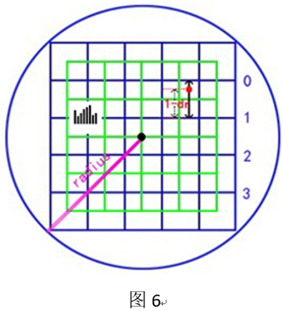
In Figure 6, it is assumed that the position of a certain point in the neighborhood is the red point in the figure, in the r dimension, it is between the 0th row and the 1st row, so its pair [0,3] and [1,3 ] Both small windows contribute. Considering only the r dimension, assuming that the fractional part of r is dr, the larger the dr, the more it deviates from row 0, the smaller the contribution to row 0, and the greater the contribution to row 1. So according to the distance, using linear interpolation, the contribution of the red point to row 0 is C0=(1-dr)*m, and the contribution to row 1 is C1=dr*m.
Then, considering the c dimension, the red point is still between the second column and the third column, so use the same method to interpolate the contributions of C0 and C1 in the column dimension to obtain C00, C01 and C10, C11 (note , where subscript 0 represents the subscript after rounding down, and 1 represents the subscript after rounding up).
Then, consider the direction group o dimension again, and obtain C000, C001...C110, C111 in sequence, with a total of 3 dimensions and 8 components.
After the above, the gradient magnitude is allocated to 4×4×8.
6.5 Normalization
The purpose of normalization is to ensure the brightness invariance of the algorithm. The normalization formula is as follows:
Among them, h is the 128-dimensional vector calculated in the previous section. In the code of Rmislam[6], the norm is used. At the same time, in order to eliminate the influence of the maximum value, according to the literature [2], Lowe sets the component whose threshold exceeds 0.2 in the normalization vector to 0.2.
6.6 python code
#################################################### 5. 计算关键点的特征描述符 #############################################
def get_descriptor(kps,gau_pyr,win_N=4, num_bins=8, scale_multiplier=3, des_max_value=0.2):
	descriptors = []
	for kp in kps:
		octave, layer  =kp.octave & 255 , (kp.octave >> 8)&255
		image = gau_pyr[octave][layer]
		img_rows,img_cols = image.shape
		bins_per_degree = num_bins / 360.
		angle = 360. - kp.angle #旋转角度为关键点方向角的负数
		cos_angle = np.cos(np.deg2rad(angle))
		sin_angle = np.sin(np.deg2rad(angle))
		weight_multiplier = -0.5 / ((0.5 * win_N) ** 2)#高斯加权运算,方差为0.5×d
		row_bin_list = []#存放每个邻域点对应4×4个小窗口中的哪一个(行)
		col_bin_list = []#存放每个邻域点对应4×4个小窗口中的哪一个(列)
		magnitude_list = []#存放每个邻域点的梯度幅值
		orientation_bin_list = []#存放每个邻域点的梯度方向角所处的方向组
		histogram_tensor = np.zeros((win_N + 2, win_N + 2, num_bins))#存放4×4×8个描述符,但为防止计算时边界溢出,在行、列的首尾各扩展一次

		hist_width = scale_multiplier * kp.size/(2**(octave)) # 3×sigma,每个小窗口的边长
		radius = int(round(hist_width * np.sqrt(2) * (win_N + 1) * 0.5))
		radius = int(min(radius, np.sqrt(img_rows ** 2 + img_cols ** 2)))

		for row in range(-radius, radius + 1):
			for col in range(-radius, radius + 1):
				row_rot = col * sin_angle + row * cos_angle#计算旋转后的坐标
				col_rot = col * cos_angle - row * sin_angle#计算旋转后的坐标
				row_bin = (row_rot / hist_width) + 0.5 * win_N - 0.5 #对应4×4子区域的下标(行)
				col_bin = (col_rot / hist_width) + 0.5 * win_N - 0.5#对应在4×4子区域的下标(列)
				if row_bin > -1 and row_bin < win_N and col_bin > -1 and col_bin < win_N:#邻域的点在旋转后,仍然处于4×4的区域内,
					window_row = int(round(kp.pt[1]*image.shape[0] + row))#计算对应原图的row
					window_col = int(round(kp.pt[0]*image.shape[1] + col))#计算对应原图的col
					if window_row > 0 and window_row < img_rows - 1 and window_col > 0 and window_col < img_cols - 1:
						dx = image[window_row, window_col + 1] - image[window_row, window_col - 1]#直接在旋转前的图上计算梯度,因为旋转时,都旋转了,不影响大小
						dy = image[window_row - 1, window_col] - image[window_row + 1, window_col]#直接在旋转前的图上计算梯度,因为旋转时,都旋转了,不影响大小
						gradient_magnitude = np.sqrt(dx * dx + dy * dy)
						gradient_orientation = np.rad2deg(np.arctan2(dy, dx)) % 360
						weight = np.exp(weight_multiplier * ((row_rot / hist_width) ** 2 + (col_rot / hist_width) ** 2))#不明白为什么要处以小窗口的边长,是要以边长为单位?
						row_bin_list.append(row_bin)
						col_bin_list.append(col_bin)
						magnitude_list.append(weight * gradient_magnitude)
						orientation_bin_list.append((gradient_orientation - angle) * bins_per_degree)#因为梯度角是旋转前的,所以还要叠加上旋转的角度

		#将magnitude分配到4*4*8(d*d*num_bins)的各区域中,即分配到histogram_tensor数组中
		for r,c,o,m in zip(row_bin_list,col_bin_list,orientation_bin_list,magnitude_list):
			ri,ci,oi = np.floor([r,c,o]).astype(int)
			rf,cf,of = [r,c,o]-np.array([ri,ci,oi])	#rf越大,越偏离当前行,同理cf,of
			#先按行分解
			c0 = m*(1-rf)#当前行的分量
			c1 = m*rf #下一行的分量
			#对每一个行分量,按列分解
			c00 = c0*(1-cf)#当前行、当前列
			c01 = c0*cf##当前行、下一列
			c10 = c1*(1-cf)#下一行、当前列
			c11=c1*cf#下一行、下一列
			#对每一个行+列分量,按方向角分解
			c000, c001 = c00*(1-of),c00*of
			c010, c011= c01*(1-of),c01*of
			c100,c101 = c10*(1-of), c10*of
			c110,c111 = c11*(1-of),c11*of
			# 数值填入到数组中
			histogram_tensor[ri+1,ci+1,oi] += c000
			histogram_tensor[ri + 1, ci + 1, (oi+1)%num_bins] += c001
			histogram_tensor[ri + 1, ci + 2, oi] += c010
			histogram_tensor[ri + 1, ci + 2, (oi + 1) % num_bins] += c011
			histogram_tensor[ri + 2, ci + 1, oi] += c100
			histogram_tensor[ri + 2, ci + 1, (oi + 1) % num_bins] += c101
			histogram_tensor[ri + 2, ci + 2, oi] += c110
			histogram_tensor[ri + 2, ci + 2, (oi + 1) % num_bins] += c111

		des_vec = histogram_tensor[1:-1,1:-1,:].flatten()#转成一维向量形式
		#des_vec[des_vec > des_max_value*np.linalg.norm(des_vec)] = des_max_value*np.linalg.norm(des_vec)
		#des_vec = des_vec / np.linalg.norm(des_vec)
		des_vec = des_vec/np.linalg.norm(des_vec)
		des_vec[des_vec>des_max_value] = des_max_value
		des_vec = np.round(512*des_vec)
		des_vec[des_vec<0]=0
		des_vec[des_vec>255]=255
		descriptors.append(des_vec)
	return descriptors
def sort_method(kp1:cv2.KeyPoint,kp2:cv2.KeyPoint):
	if kp1.pt[0] != kp2.pt[0]:
		return kp1.pt[0] - kp2.pt[0]
	if kp1.pt[1] != kp2.pt[1]:
		return kp1.pt[1] - kp2.pt[1]
	if kp1.size != kp2.size:
		return kp1.size - kp2.size
	if kp1.angle != kp2.angle:
		return kp1.angle - kp2.angle
	if kp1.response != kp2.response:
		return kp1.response - kp2.response
	if kp1.octave != kp2.octave:
		return kp1.octave - kp2.octave
	return kp1.class_id - kp2.class_id
def remove_duplicate_points(keypoints):
	keypoints.sort(key=cmp_to_key(sort_method))
	unique_keypoints = [keypoints[0]]

	for next_keypoint in keypoints[1:]:
		last_unique_keypoint = unique_keypoints[-1]
		if last_unique_keypoint.pt[0] != next_keypoint.pt[0] or \
				last_unique_keypoint.pt[1] != next_keypoint.pt[1] or \
				last_unique_keypoint.size != next_keypoint.size or \
				last_unique_keypoint.angle != next_keypoint.angle:
			unique_keypoints.append(next_keypoint)
	return unique_keypoints
7. Matching of Feature Descriptors
After the processing in the previous section, the feature descriptors of the key points of the image are obtained. After obtaining the key point feature descriptors of the two images, descriptor matching can be performed. For two key point descriptors, judge whether the matching is successful or not by judging the size of the Euclidean distance [2]; for all key point descriptors of the two images, use exhaustive matching or cluster matching.
Use opencv's FlannBasedMatcher.knnMatch() function to match the feature descriptors of the two images. The usage of this function, reference [9] and the comment area of [9] (the experts are all in the comment area).
The Python code is as follows:
#################################################### 6. 匹配 ############################################################
def do_match(img_src1,kp1,des1,img_src2,kp2,des2,embed=1,pt_flag=0,MIN_MATCH_COUNT = 10):
	## 1. 对关键点进行匹配 ##
	FLANN_INDEX_KDTREE = 0
	index_params = dict(algorithm=FLANN_INDEX_KDTREE, trees=5)
	search_params = dict(checks=50)
	flann = cv2.FlannBasedMatcher(index_params, search_params)
	des1, des2 = np.array(des1).astype(np.float32), np.array(des2).astype(np.float32)#需要转成array
	matches = flann.knnMatch(des1, des2, k=2)  # matches为list,每个list元素由2个DMatch类型变量组成,分别是最邻近和次邻近点

	good_match = []
	for m in matches:
		if m[0].distance < 0.7 * m[1].distance:  # 如果最邻近和次邻近的距离差距较大,则认可
			good_match.append(m[0])
	## 2. 将2张图画在同一张图上 ##
	img1 = img_src1.copy()
	img2 = img_src2.copy()
	h1, w1 = img1.shape[0],img1.shape[1]
	h2, w2 = img2.shape[0],img2.shape[1]
	new_w = w1 + w2
	new_h = np.max([h1, h2])
	new_img =  np.zeros((new_h, new_w,3), np.uint8) if len(img_src1.shape)==3 else  np.zeros((new_h, new_w), np.uint8)
	h_offset1 = int(0.5 * (new_h - h1))
	h_offset2 = int(0.5 * (new_h - h2))
	if len(img_src1.shape) == 3:
		new_img[h_offset1:h_offset1 + h1, :w1,:] = img1  # 左边画img1
		new_img[h_offset2:h_offset2 + h2, w1:w1 + w2,:] = img2  # 右边画img2
	else:
		new_img[h_offset1:h_offset1 + h1, :w1] = img1  # 左边画img1
		new_img[h_offset2:h_offset2 + h2, w1:w1 + w2] = img2  # 右边画img2
	##3. 两幅图存在足够的匹配点,两幅图匹配成功,将匹配成功的关键点进行连线 ##
	if len(good_match) > MIN_MATCH_COUNT:
		src_pts = []
		dst_pts = []
		mag_err_arr=[]
		angle_err_arr=[]
		for m in good_match:
			if pt_flag==0:#point是百分比
				src_pts.append([kp1[m.queryIdx].pt[0] * img1.shape[1], kp1[m.queryIdx].pt[1] * img1.shape[0]])#保存匹配成功的原图关键点位置
				dst_pts.append([kp2[m.trainIdx].pt[0] * img2.shape[1], kp2[m.trainIdx].pt[1] * img2.shape[0]])#保存匹配成功的目标图关键点位置
			else:
				src_pts.append([kp1[m.queryIdx].pt[0], kp1[m.queryIdx].pt[1]])  # 保存匹配成功的原图关键点位置
				dst_pts.append([kp2[m.trainIdx].pt[0], kp2[m.trainIdx].pt[1]])  # 保存匹配成功的目标图关键点位置

			mag_err = np.abs(kp1[m.queryIdx].response - kp2[m.trainIdx].response) / np.abs(kp1[m.queryIdx].response )
			angle_err = np.abs(kp1[m.queryIdx].angle - kp2[m.trainIdx].angle)
			mag_err_arr.append(mag_err)
			angle_err_arr.append(angle_err)

		if embed!=0 :#若图像2是图像1内嵌入另一个大的背景中,则在图像2中,突出显示图像1的边界
			M = cv2.findHomography(np.array(src_pts), np.array(dst_pts), cv2.RANSAC, 5.0)[0]  # 根据src和dst关键点,寻求变换矩阵
			src_w, src_h = img1.shape[1], img1.shape[0]
			src_rect = np.array([[0, 0], [src_w - 1, 0], [src_w - 1, src_h - 1], [0, src_h - 1]]).reshape(-1, 1, 2).astype(
				np.float32)  # 原始图像的边界框
			dst_rect = cv2.perspectiveTransform(src_rect, M)  # 经映射后,得到dst的边界框
			img2 = cv2.polylines(img2, [np.int32(dst_rect)], True, 255, 3, cv2.LINE_AA)  # 将边界框画在dst图像上,突出显示
			if len(new_img.shape) == 3:
				new_img[h_offset2:h_offset2 + h2, w1:w1 + w2,:] = img2  # 右边画img2
			else:
				new_img[h_offset2:h_offset2 + h2, w1:w1 + w2] = img2  # 右边画img2

		new_img = new_img if len(new_img.shape) == 3 else  cv2.cvtColor(new_img, cv2.COLOR_GRAY2BGR)
		# 连线
		for pt1, pt2 in zip(src_pts, dst_pts):
			cv2.line(new_img, tuple(np.int32(np.array(pt1) + [0, h_offset1])),
					 tuple(np.int32(np.array(pt2) + [w1, h_offset2])), color=(0, 0, 255))
	return new_img
8. Test Results
python program:
def do_sift(img_src,sift:CSift):
	img = img_src.copy().astype(np.float32)
	img = pre_treat_img(img,sift.sigma)
	sift.num_octave = get_numOfOctave(img)
	gaussian_pyr = construct_gaussian_pyramid(img,sift)
	dog_pyr = construct_DOG(gaussian_pyr)
	key_points = get_keypoints(gaussian_pyr,dog_pyr,sift)
	key_points = remove_duplicate_points(key_points)
	descriptor = get_descriptor(key_points,gaussian_pyr)
	return key_points,descriptor
if __name__ == '__main__':
	MIN_MATCH_COUNT = 10
	sift = CSift(num_octave=4,num_scale=3,sigma=1.6)
	img_src1 = cv2.imread('box.png',-1)
	#img_src1 = cv2.resize(img_src1, (0, 0), fx=.25, fy=.25)
	img_src2 = cv2.imread('box_in_scene.png', -1)
	#img_src2 = cv2.resize(img_src2, (0, 0), fx=.5, fy=.5)
	# 1. 使用本sift算子
	kp1, des1 = do_sift(img_src1, sift)
	kp2, des2 = do_sift(img_src2, sift)
	pt_flag = 0
	'''
	# 3. 做匹配
	reu_img = do_match(img_src1, kp1, des1, img_src2, kp2, des2, embed=1, pt_flag=pt_flag,MIN_MATCH_COUNT=3)
	cv2.imshow('reu',reu_img)
	cv2.imwrite('reu.tif',reu_img)
Note: It takes a long time to run, very slow, very slow, just like the previous carriages and horses, please be patient.
Test with box image
9. Implementation of SIFT based on opencv
The SIFT algorithm is integrated in Opencv. Here, the Opencv-python version used is 4.4.0.42. The method of use is 3 steps:
opencv_sift = cv2.SIFT.create(nfeatures=None, nOctaveLayers= None,
                       contrastThreshold= None, edgeThreshold= None , sigma= None )
kp1 = opencv_sift.detect(img_src1)
kp1,des1 = opencv_sift.compute(img_src1,kp1)
When creating an operator, fill in the relevant parameters. The sift operator that comes with Opencv is super fast, and the results obtained are more than manually written (may be related to parameters). The returned kp is the keypoint class, which contains information such as the position, orientation, and response value (gradient value) of each key point.
python code:
if __name__ == '__main__':
	MIN_MATCH_COUNT = 10
	sift = CSift(num_octave=4,num_scale=3,sigma=1.6)
	img_src1 = cv2.imread('box.png',-1)
	#img_src1 = cv2.resize(img_src1, (0, 0), fx=.25, fy=.25)
	img_src2 = cv2.imread('box_in_scene.png', -1)
	#img_src2 = cv2.resize(img_src2, (0, 0), fx=.5, fy=.5)
	# 2. 使用opencv自带sift算子
	sift.num_octave = get_numOfOctave(img_src1)
	opencv_sift = cv2.SIFT.create(nfeatures=None, nOctaveLayers=sift.num_octave,
								  contrastThreshold=sift.contrast_t, edgeThreshold=sift.eigenvalue_r, sigma=sift.sigma)
	kp1 = opencv_sift.detect(img_src1)
	kp1,des1 = opencv_sift.compute(img_src1,kp1)

	sift.num_octave = get_numOfOctave(img_src2)
	opencv_sift = cv2.SIFT.create(nfeatures=None, nOctaveLayers=sift.num_octave,
								  contrastThreshold=sift.contrast_t, edgeThreshold=sift.eigenvalue_r, sigma=sift.sigma)
	kp2 = opencv_sift.detect(img_src2)
	kp2, des2 = opencv_sift.compute(img_src2, kp2)
	pt_flag = 1

	# 3. 做匹配
	reu_img = do_match(img_src1, kp1, des1, img_src2, kp2, des2, embed=1, pt_flag=pt_flag,MIN_MATCH_COUNT=3)
	cv2.imshow('reu',reu_img)
	cv2.imwrite('reu.tif',reu_img)
Test results:

So, uh uh, why do you have to write the code yourself, why bother with yourself.
10. about the question
The camera is placed on the ground at a constant height from the ceiling. Take a picture against the ceiling at a certain position, then move the camera a certain distance, rotate a certain angle, and then take another picture. Are the feature points on these two pictures consistent in gradient value and gradient direction?
10.1 Only rotate a certain angle and the camera is horizontal
On the premise that the camera is horizontal, if the camera is only rotated by a certain angle, theoretically, the second picture is also the result of the first picture rotated by this angle. Therefore, the magnitude of the gradient value of the feature points on the two images will not change, but the direction of the gradient will change, and the difference is the rotation angle.
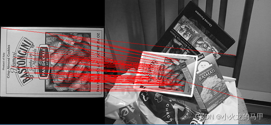
Use a picture for a rotation test. In order to prevent opencv from changing the pixel value caused by interpolation of the image when rotating the image, here, the rotation angle is 90 degrees, and the rotation is performed directly using matrix operations. Call opencv's sift algorithm on the two images to obtain key points and descriptors, and then perform matching. During the matching process, the error in the gradient value and gradient direction of the key point of successful matching is saved, the gradient value error is a relative error, and the gradient direction error is an absolute error. The result is shown in the figure below.
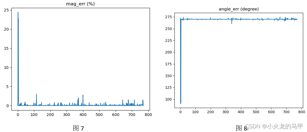
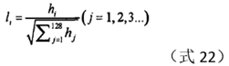
It can be seen from the test results that the gradient amplitude error is basically within 2%, and the gradient direction error is basically around 270 degrees. In Figures 7 and 8, the 2nd and 4th points have obvious abnormal jumps, and the reason is to find out: when the key points are matched, the matching is misplaced, as shown in Figure 9.

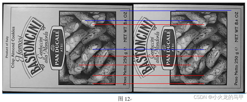
In Figure 9, the blue lines are the 2 with the largest gradient value errors; the red lines are the 5 with the smallest gradient value errors. It can be seen that the position point matching error occurs on the blue line, so there will naturally be a large error in the gradient value.
10.2 Only move a certain distance and the camera is horizontal
On the premise that the camera is horizontal, the distance the camera moves is equivalent to moving out the old scene and moving in the new scene. At this time, the gradient value and gradient direction of the key points are theoretically unchanged in the two images before and after.
Use images for moving in and out testing, and use matrix operations directly without changing pixel values. The two images were processed in the same way as in the previous section. The result is shown in the figure below.
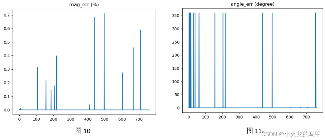
It can be seen that the gradient value error is very small, and the gradient direction is consistent (0 or 360 degrees).
10.3 The camera is not level
If the camera is not absolutely horizontal in the field of view (for example, there is an angle of inclination to the ceiling), the camera movement and rotation should all cause changes in the gradient value, because the pixels around the key point have changed, and the gradient value is computed. The comprehensive result of all neighborhoods within the radius of the extreme point r, this r is also related to the scale. How much the change of the gradient value affects is related to the level of the camera, the moving distance, and the rotation angle.
Use affine transformation to simulate the imaging after the camera is moved and rotated when it is not horizontal. The two images were processed in the same way as in the previous section. The result is shown in the figure below.

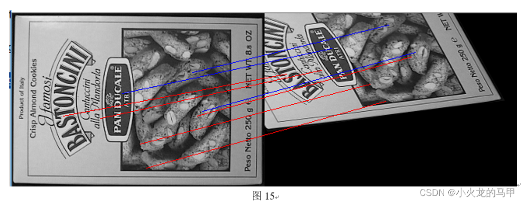
It can be seen that the error of the gradient value becomes significantly larger. But this can't explain anything exactly. After all, when performing affine transformation, interpolation processing has been performed to modify the image pixels. In addition, whether the matching of key points is accurate also needs to be considered.
The python code tested in this section:
#################################################### 7. 测试移动和旋转 ####################################################
def move_rotate_sift_test():
	img_src = cv2.imread('box.png', 0)
	img_src1 = img_src.copy()
	#### 情形1.旋转90度 ###
	img_src2 = img_src1.transpose()
	img_src2 = np.fliplr(img_src2)
	#### 情形2. 景色移出视野 ###
	img_src2 = img_src1[:,50:]
	#### 情形3. 放射变换 ###
	points1 = np.float32([[81, 30], [378, 80], [13, 425]])
	points2 = np.float32([[0, 0], [300, 0], [100, 300]])
	affine_matrix = cv2.getAffineTransform(points1, points2)

	img_src2 = cv2.warpAffine(img_src1, affine_matrix, (0, 0), flags=cv2.INTER_CUBIC,
							  borderMode=cv2.BORDER_CONSTANT, borderValue=0)

	#### 做sift ####
	sift.num_octave = get_numOfOctave(img_src1)
	opencv_sift = cv2.SIFT.create(nfeatures=None, nOctaveLayers=sift.num_octave,
								  contrastThreshold=sift.contrast_t, edgeThreshold=sift.eigenvalue_r, sigma=sift.sigma)
	kp1 = opencv_sift.detect(img_src1)
	kp1, des1 = opencv_sift.compute(img_src1, kp1)

	sift.num_octave = get_numOfOctave(img_src2)
	opencv_sift = cv2.SIFT.create(nfeatures=None, nOctaveLayers=sift.num_octave,
								  contrastThreshold=sift.contrast_t, edgeThreshold=sift.eigenvalue_r, sigma=sift.sigma)
	kp2 = opencv_sift.detect(img_src2)
	kp2, des2 = opencv_sift.compute(img_src2, kp2)

	reu_img = do_match_compare(img_src1, kp1, des1, img_src2, kp2, des2, embed=0, pt_flag=1, MIN_MATCH_COUNT=3)
	cv2.imshow('reu', reu_img)


	return
def do_match_compare(img_src1,kp1,des1,img_src2,kp2,des2,embed=1,pt_flag=0,MIN_MATCH_COUNT = 10):
	## 1. 对关键点进行匹配 ##
	FLANN_INDEX_KDTREE = 0
	index_params = dict(algorithm=FLANN_INDEX_KDTREE, trees=5)
	search_params = dict(checks=50)
	flann = cv2.FlannBasedMatcher(index_params, search_params)
	des1, des2 = np.array(des1).astype(np.float32), np.array(des2).astype(np.float32)#需要转成array
	matches = flann.knnMatch(des1, des2, k=2)  # matches为list,每个list元素由2个DMatch类型变量组成,分别是最邻近和次邻近点

	good_match = []
	for m in matches:
		if m[0].distance < 0.5 * m[1].distance:  # 如果最邻近和次邻近的距离差距较大,则认可
			good_match.append(m[0])
	## 2. 将2张图画在同一张图上 ##
	img1 = img_src1.copy()
	img2 = img_src2.copy()
	h1, w1 = img1.shape[0],img1.shape[1]
	h2, w2 = img2.shape[0],img2.shape[1]
	new_w = w1 + w2
	new_h = np.max([h1, h2])
	new_img = np.zeros((new_h, new_w), np.uint8)
	h_offset1 = int(0.5 * (new_h - h1))
	h_offset2 = int(0.5 * (new_h - h2))
	new_img[h_offset1:h_offset1 + h1, :w1] = img1  # 左边画img1
	new_img[h_offset2:h_offset2 + h2, w1:w1 + w2] = img2  # 右边画img2
	##3. 两幅图存在足够的匹配点,两幅图匹配成功,将匹配成功的关键点进行连线 ##
	if len(good_match) > MIN_MATCH_COUNT:
		src_pts = []
		dst_pts = []
		mag_err_arr=[] #保存匹配的关键点,在梯度幅值上的相对误差
		angle_err_arr=[]#保存匹配的关键点,在梯度方向上的绝对误差
		for m in good_match:
			if pt_flag==0:#point是百分比
				src_pts.append([kp1[m.queryIdx].pt[0] * img1.shape[1], kp1[m.queryIdx].pt[1] * img1.shape[0]])#保存匹配成功的原图关键点位置
				dst_pts.append([kp2[m.trainIdx].pt[0] * img2.shape[1], kp2[m.trainIdx].pt[1] * img2.shape[0]])#保存匹配成功的目标图关键点位置
			else:
				src_pts.append([kp1[m.queryIdx].pt[0], kp1[m.queryIdx].pt[1]])  # 保存匹配成功的原图关键点位置
				dst_pts.append([kp2[m.trainIdx].pt[0], kp2[m.trainIdx].pt[1]])  # 保存匹配成功的目标图关键点位置

			mag_err = np.abs(kp1[m.queryIdx].response - kp2[m.trainIdx].response) / np.abs(kp1[m.queryIdx].response ) *100
			angle_err = (kp1[m.queryIdx].angle - kp2[m.trainIdx].angle)%360
			mag_err_arr.append(mag_err)
			angle_err_arr.append(angle_err)
		new_img = cv2.cvtColor(new_img, cv2.COLOR_GRAY2BGR)
		plt.figure()
		plt.title('mag_err (%)')
		plt.plot(mag_err_arr)

		plt.figure()
		plt.title('angle_err (degree)')
		plt.plot(angle_err_arr)
		plt.show()
		# 连线
		index = np.argsort(mag_err_arr)#进行有小到大排序

		for i in range(0,5): #画出误差最小的5个匹配点连线
			pt1, pt2 = src_pts[index[i]], dst_pts[index[i]]
			cv2.line(new_img, tuple(np.int32(np.array(pt1) + [0, h_offset1])),
					 tuple(np.int32(np.array(pt2) + [w1, h_offset2])), color=(0, 0, 255))
		for i in range(-3, 0):#画出误差最大的3个匹配点连线
			pt1, pt2 = src_pts[index[i]], dst_pts[index[i]]
			cv2.line(new_img, tuple(np.int32(np.array(pt1) + [0, h_offset1])), tuple(np.int32(np.array(pt2) + [w1, h_offset2])), color=(255, 0, 0))
	return new_img
11. Source code download
https://download.csdn.net/download/xiaohuolong1827/85221790
12. other
Use other pictures for testing.
On the left is Huang Ningran who went at night in February, and on the right is the author who went during the day in April. Been where you've been, seen what you've seen. So what about the matching results?
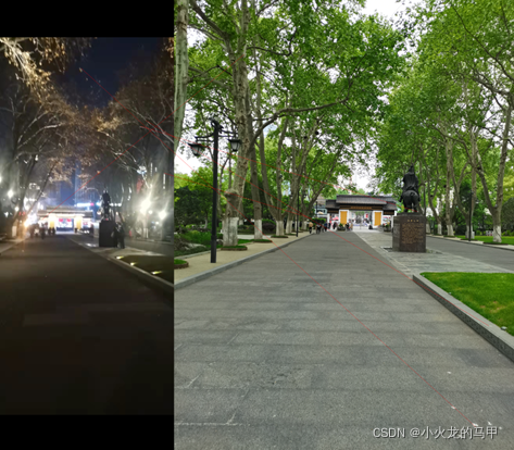
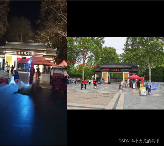
Uh, GG. Still need to read more.
This post, right when happy.