Wisdom target detection 65 - Pytorch builds DETR target detection platform
- study preface
- Source code download
- DETR implementation ideas
- Train your own DETR model
study preface
Transformer-based target detection has not been done, make up for it.

Source code download
https://github.com/bubbliiiiing/detr-pytorch
If you like it, you can order a star.
DETR implementation ideas
1. Overall structure analysis

Before learning DETR, we need to have a certain understanding of what DETR does, which will help us understand the details of the network later. The picture above is Fig. 2 in the paper, which better shows the working principle of the whole DETR. The whole DETR can be divided into four parts, namely: backbone, encoder, decoder and prediction heads .
Backbone is the backbone feature extraction network of DETR . The input image will first be feature extracted in the backbone network . The extracted features can be called the feature layer, which is the feature set of the input image . In the backbone part, we obtained a feature layer for the next step of network construction. I call this feature layer an effective feature layer .
Encoder is Transformer's encoding network-feature enhancement . An effective feature layer obtained in the backbone part will first be tiled in the height and width dimensions to become a feature sequence, and then continue to use Self-Attension in this part to enhance feature extraction and obtain An enhanced effective feature layer . It belongs to the encoding network of Transformer, and the next step of encoding is decoding.
Decoder is Transformer's decoding network-feature query . An enhanced effective feature layer obtained in the encoder part will be decoded in this part. Decoding requires the use of a very important learnable module, that is, the object queries shown in the above figure. In the decoder part, we use a learnable query vector q to query the enhanced effective feature layer to obtain prediction results.
The prediction heads are the classifier and regressor of DETR . In fact, they are fully connected to the prediction results obtained by the decoder. The two full connections represent the category and regression parameters respectively. There are 4 FFNs drawn on the picture, and 2 FFNs in the source code.
Therefore, the work done by the entire DETR network is feature extraction-feature enhancement-feature query-prediction results .
2. Analysis of network structure
1. Introduction to backbone network Backbone
DETR can use a variety of backbone feature extraction networks. Resnet is used in the paper. This article uses the Resnet50 network as an example to demonstrate it to everyone.
a. What is a residual network
Residual net (residual network): The data output
of a certain layer of the first few layers is directly skipped over multiple layers and introduced into the input part of the subsequent data layer.
It means that part of the content of the following feature layer will be linearly contributed by a layer in front of it.
Its structure is as follows:

the design of the deep residual network is to overcome the problems of low learning efficiency and ineffective improvement of accuracy due to the deepening of the network depth.
b. What is the ResNet50 model
ResNet50 has two basic blocks, namely Conv Block and Identity Block. The input and output dimensions of the Conv Block are different, so they cannot be connected in series. Its function is to change the dimension of the network; the input dimension and output of the Identity Block The dimensions are the same and can be connected in series, and its function is to deepen the network.
The structure of the Conv Block is as follows. As can be seen from the figure, the Conv Block can be divided into two parts. The left part is the main part. There are two convolutions, normalization, activation function and one convolution and standardization; the right part is the residual edge. Part, there is a convolution and normalization , because there is convolution in the residual side, so we can use the Conv Block to change the width, height and channel number of the output feature layer: The
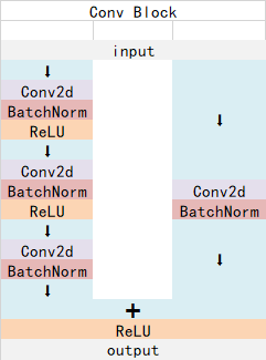
structure of the Identity Block is as follows, as can be seen from the figure, the Identity Block can It is divided into two parts, the left part is the main part, there are two convolutions, normalization, activation function and one convolution and standardization; the right part is the residual edge part, which is directly connected to the output, because the residual edge part does not exist Convolution, so the shape of the input feature layer and the output feature layer of the Identity Block are the same, which can be used to deepen the network:

Conv Block and Identity Block are both residual network structures.
The overall network structure is as follows:

In DETR, suppose the input is [batch_size, 3, 800, 800], and the output is [batch_size, 2048, 25, 25], the code directly uses the resnet that comes with the torchvision library, so The entire backbone implementation code is:
class FrozenBatchNorm2d(torch.nn.Module):
    """
    冻结固定的BatchNorm2d。
    """
    def __init__(self, n):
        super(FrozenBatchNorm2d, self).__init__()
        self.register_buffer("weight", torch.ones(n))
        self.register_buffer("bias", torch.zeros(n))
        self.register_buffer("running_mean", torch.zeros(n))
        self.register_buffer("running_var", torch.ones(n))

    def _load_from_state_dict(self, state_dict, prefix, local_metadata, strict, missing_keys, unexpected_keys, error_msgs):
        num_batches_tracked_key = prefix + 'num_batches_tracked'
        if num_batches_tracked_key in state_dict:
            del state_dict[num_batches_tracked_key]

        super(FrozenBatchNorm2d, self)._load_from_state_dict(
            state_dict, prefix, local_metadata, strict,
            missing_keys, unexpected_keys, error_msgs)

    def forward(self, x):
        w       = self.weight.reshape(1, -1, 1, 1)
        b       = self.bias.reshape(1, -1, 1, 1)
        rv      = self.running_var.reshape(1, -1, 1, 1)
        rm      = self.running_mean.reshape(1, -1, 1, 1)
        eps     = 1e-5
        scale   = w * (rv + eps).rsqrt()
        bias    = b - rm * scale
        return x * scale + bias

class BackboneBase(nn.Module):
    """
    用于指定返回哪个层的输出
    这里返回的是最后一层
    """
    def __init__(self, backbone: nn.Module, train_backbone: bool, num_channels: int, return_interm_layers: bool):
        super().__init__()
        for name, parameter in backbone.named_parameters():
            if not train_backbone or 'layer2' not in name and 'layer3' not in name and 'layer4' not in name:
                parameter.requires_grad_(False)
        if return_interm_layers:
            return_layers   = {

    "layer1": "0", "layer2": "1", "layer3": "2", "layer4": "3"}
        else:
            return_layers   = {

    'layer4': "0"}

        # 用于指定返回的层
        self.body           = IntermediateLayerGetter(backbone, return_layers=return_layers)
        self.num_channels   = num_channels

    def forward(self, tensor_list: NestedTensor):
        xs                           = self.body(tensor_list.tensors)
        out: Dict[str, NestedTensor] = {

    }
        for name, x in xs.items():
            m           = tensor_list.mask
            assert m is not None
            mask        = F.interpolate(m[None].float(), size=x.shape[-2:]).to(torch.bool)[0]
            out[name]   = NestedTensor(x, mask)
        return out

class Backbone(BackboneBase):
    """
    ResNet backbone with frozen BatchNorm.
    """
    def __init__(self, name: str, train_backbone: bool, return_interm_layers: bool,dilation: bool):
        # 首先利用torchvision里面的model创建一个backbone模型
        backbone = getattr(torchvision.models, name)(
            replace_stride_with_dilation    = [False, False, dilation],
            pretrained                      = is_main_process(),
            norm_layer                      = FrozenBatchNorm2d
        )
        # 根据选择的模型,获得通道数
        num_channels = 512 if name in ('resnet18', 'resnet34') else 2048
        super().__init__(backbone, train_backbone, num_channels, return_interm_layers)
c. Position code

In addition to using the backbone for feature extraction, because the Transformer needs to be passed in for feature extraction and feature query, the features obtained by the backbone also need to be position coded. It does not belong to the backbone in the picture, but it is implemented in backbone.py, so let's briefly analyze it together.
In fact, it is the idea of the position embedding of the original Transformer, which adds position information to all features , so that the network has the ability to distinguish different regions .
DETR calculates a position code for the feature map output by resnet in the pos_x and pos_y directions respectively. The position code length of each dimension is num_pos_feats, which defaults to half of the Transformer's feature length, which is 128. For pos_x and pos_y, the sine is calculated at the odd position, the cosine is calculated at the even position, and then the calculation results are spliced. Get a vector of [batch_size, h, w, 256]. Finally, transpose to obtain a vector of [batch_size, 256, h, w].
code show as below:
class PositionEmbeddingSine(nn.Module):
    """
    这是一个更标准的位置嵌入版本,按照sine进行分布
    """
    def __init__(self, num_pos_feats=64, temperature=10000, normalize=False, scale=None):
        super().__init__()
        self.num_pos_feats  = num_pos_feats
        self.temperature    = temperature
        self.normalize      = normalize
        if scale is not None and normalize is False:
            raise ValueError("normalize should be True if scale is passed")
        if scale is None:
            scale = 2 * math.pi
        self.scale = scale

    def forward(self, tensor_list: NestedTensor):
        x           = tensor_list.tensors
        mask        = tensor_list.mask
        assert mask is not None
        not_mask    = ~mask
        y_embed     = not_mask.cumsum(1, dtype=torch.float32)
        x_embed     = not_mask.cumsum(2, dtype=torch.float32)
        if self.normalize:
            eps     = 1e-6
            y_embed = y_embed / (y_embed[:, -1:, :] + eps) * self.scale
            x_embed = x_embed / (x_embed[:, :, -1:] + eps) * self.scale

        dim_t = torch.arange(self.num_pos_feats, dtype=torch.float32, device=x.device)
        dim_t = self.temperature ** (2 * (dim_t // 2) / self.num_pos_feats)

        pos_x = x_embed[:, :, :, None] / dim_t
        pos_y = y_embed[:, :, :, None] / dim_t
        pos_x = torch.stack((pos_x[:, :, :, 0::2].sin(), pos_x[:, :, :, 1::2].cos()), dim=4).flatten(3)
        pos_y = torch.stack((pos_y[:, :, :, 0::2].sin(), pos_y[:, :, :, 1::2].cos()), dim=4).flatten(3)
        pos = torch.cat((pos_y, pos_x), dim=3).permute(0, 3, 1, 2)
        return pos
2. Encoding network Encoder network introduction
a. Construction of Transformer Encoder
In the above, we obtained two matrices, one matrix is the feature matrix of the input image, and the other is the position code corresponding to the feature matrix. Their shapes are [batch_size, 2048, 25, 25], [batch_size, 256, 25, 25] respectively.
In the encoding network part, DETR uses the Encoder part of the Transformer for feature extraction. We need to first scale the channel of the feature matrix. If the feature matrix is directly extracted by the transformer, the number of channels in the network is too large (2048), which will directly lead to insufficient video memory. Use a 1x1 nn.Conv2d to compress the channel. The compressed channel is 256, which is the characteristic length used by Transformer. At this point we have obtained a feature matrix with a shape of [batch_size, 256, 25, 25].
Then we tile the feature matrix and the height and width dimensions of the position code to obtain two matrices with a shape of [batch_size, 256, 625]. Since we use the nn.MultiheadAttention that comes with Pytorch, this module requires batch_size to be at the first dimension, the sequence length is in the 0th dimension, so we transpose the feature matrix and the position code, and the two transposed matrices are [625, batch_size, 256].
We can now input it into the Encoder for feature extraction. The Encoder does not change the shape of the input, so the enhanced feature sequence shape after feature extraction by the Encoder is also [625, batch_size, 256].
Since in DETR, Transformer's Encoder directly uses Pytorch's MultiheadAttention, we don't have to worry too much about the principle, just understand it briefly. In DETR, the implementation code of the entire Transformer Encoder is:
class TransformerEncoder(nn.Module):
    def __init__(self, encoder_layer, num_layers, norm=None):
        super().__init__()
        self.layers = _get_clones(encoder_layer, num_layers)
        self.num_layers = num_layers
        self.norm = norm

    def forward(self, src,
                mask: Optional[Tensor] = None,
                src_key_padding_mask: Optional[Tensor] = None,
                pos: Optional[Tensor] = None):
        output = src
        # 625, batch_size, 256 => ...(x6)... => 625, batch_size, 256
        for layer in self.layers:
            output = layer(output, src_mask=mask, src_key_padding_mask=src_key_padding_mask, pos=pos)

        if self.norm is not None:
            output = self.norm(output)
        return output

class TransformerEncoderLayer(nn.Module):
    def __init__(self, d_model, nhead, dim_feedforward=2048, dropout=0.1,
                 activation="relu", normalize_before=False):
        super().__init__()
        # Self-Attention模块
        self.self_attn  = nn.MultiheadAttention(d_model, nhead, dropout=dropout)
        # FFN模块
        # Implementation of Feedforward model
        self.linear1    = nn.Linear(d_model, dim_feedforward)
        self.dropout    = nn.Dropout(dropout)
        self.linear2    = nn.Linear(dim_feedforward, d_model)

        self.norm1      = nn.LayerNorm(d_model)
        self.norm2      = nn.LayerNorm(d_model)
        self.dropout1   = nn.Dropout(dropout)
        self.dropout2   = nn.Dropout(dropout)

        self.activation = _get_activation_fn(activation)
        self.normalize_before = normalize_before

    def with_pos_embed(self, tensor, pos: Optional[Tensor]):
        return tensor if pos is None else tensor + pos

    def forward_post(self,
                     src,
                     src_mask: Optional[Tensor] = None,
                     src_key_padding_mask: Optional[Tensor] = None,
                     pos: Optional[Tensor] = None):
        # 添加位置信息
        # 625, batch_size, 256 => 625, batch_size, 256
        q = k = self.with_pos_embed(src, pos)
        # 使用自注意力机制模块
        # 625, batch_size, 256 => 625, batch_size, 256
        src2 = self.self_attn(q, k, value=src, attn_mask=src_mask, key_padding_mask=src_key_padding_mask)[0]
        # 添加残差结构
        # 625, batch_size, 256 => 625, batch_size, 256
        src = src + self.dropout1(src2)

        # 添加FFN结构
        # 625, batch_size, 256 => 625, batch_size, 2048 => 625, batch_size, 256
        src = self.norm1(src)
        src2 = self.linear2(self.dropout(self.activation(self.linear1(src))))
        # 添加残差结构
        # 625, batch_size, 256 => 625, batch_size, 256
        src = src + self.dropout2(src2)
        src = self.norm2(src)
        return src

    def forward_pre(self, src,
                    src_mask: Optional[Tensor] = None,
                    src_key_padding_mask: Optional[Tensor] = None,
                    pos: Optional[Tensor] = None):
        src2 = self.norm1(src)
        q = k = self.with_pos_embed(src2, pos)
        src2 = self.self_attn(q, k, value=src2, attn_mask=src_mask,
                              key_padding_mask=src_key_padding_mask)[0]
        src = src + self.dropout1(src2)
        src2 = self.norm2(src)
        src2 = self.linear2(self.dropout(self.activation(self.linear1(src2))))
        src = src + self.dropout2(src2)
        return src

    def forward(self, src,
                src_mask: Optional[Tensor] = None,
                src_key_padding_mask: Optional[Tensor] = None,
                pos: Optional[Tensor] = None):
        if self.normalize_before:
            return self.forward_pre(src, src_mask, src_key_padding_mask, pos)
        return self.forward_post(src, src_mask, src_key_padding_mask, pos)
b. Self-attention structure analysis
Here you can briefly understand the principle of the multi-head attention mechanism. The calculation principle of the multi-head attention mechanism is as follows:
To understand the Self-attention structure, in fact, it is enough to understand the animation below. There is a sequence of three unit inputs in the animation . The input of each sequence unit can be obtained through three processes (such as full connection) Query, Key, Value , Query is a query vector, Key is a key vector, and Value is a vector.

If we want to obtain the output of input-1, then we proceed as follows:
1. Use the query vector of input-1 to multiply the key vectors of input-1, input-2, and input-3 respectively . At this time, we get Got three scores .
2. Then take softmax for these three scores , and obtain the respective importance of input-1, input-2, and input-3 .
3. Then multiply this importance by the value vectors of input-1, input-2, and input-3 , and sum.
4. At this point we have obtained the output of input-1.
As shown in the figure, we carry out the following steps:
1. The query vector of input-1 is [1, 0, 2] , multiply the key vectors of input-1, input-2, and input-3 respectively to obtain three scores For 2, 4, 4.
2. Then take softmax for these three scores , and obtain the respective importance levels of input-1, input-2, and input-3 , and obtain three importance levels of 0.0, 0.5, and 0.5.
3. Then multiply this importance by the value vectors of input-1, input-2, and input-3, and sum, that is,
0.0 ∗ [ 1 , 2 , 3 ] + 0.5 ∗ [ 2 , 8 , 0 ] + 0.5 ∗ [ 2 , 6 , 3 ] = [ 2.0 , 7.0 , 1.5 ] 0.0 * [1, 2, 3] + 0.5 * [2, 8, 0] + 0.5 * [2, 6, 3] = [2.0, 7.0, 1.5]0.0∗[1,2,3]+0.5∗[2,8,0]+0.5∗[2,6,3]=[2.0,7.0,1.5 ] .
4. At this point we have obtained the output [2.0, 7.0, 1.5] of input-1.
In the above example, the sequence length is only 3, and the characteristic length of each unit sequence is only 3. In DETR's Transformer Encoder, the sequence length is 625, and the characteristic length of each unit sequence is 256 // num_heads . But the calculation process is the same. In actual operations, we use matrices for operations.
The actual matrix operation process is shown in the figure below. Let me take the actual matrix as an example to explain to you:
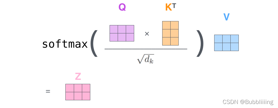
the input Query, Key, and Value are shown in the following figure:

first, use the query vector query to cross- multiply transposed key vector key . This step can be commonly understood as using the query vector to query The characteristics of the sequence, the importance score of each part of the sequence is obtained.
Each line of output represents the contribution of input-1, input-2, and input-3 to the current input . We take a softmax for this contribution value.


Then use the score to cross-multiply the value. This step can be commonly understood as reapplying the importance of each part of the sequence to the value of the sequence.

The code of this matrix operation is shown below, you can try it yourself.
import numpy as np

def soft_max(z):
    t = np.exp(z)
    a = np.exp(z) / np.expand_dims(np.sum(t, axis=1), 1)
    return a

Query = np.array([
    [1,0,2],
    [2,2,2],
    [2,1,3]
])

Key = np.array([
    [0,1,1],
    [4,4,0],
    [2,3,1]
])

Value = np.array([
    [1,2,3],
    [2,8,0],
    [2,6,3]
])

scores = Query @ Key.T
print(scores)
scores = soft_max(scores)
print(scores)
out = scores @ Value
print(out)
3. Decoder Network Decoder Network Introduction
Through the second step above, we can obtain a feature matrix that uses Encoder to enhance feature extraction, and its shape is [625, batch_size, 256].
An enhanced effective feature layer obtained in the encoder part will be decoded in this part, and decoding requires the use of a very important learnable module, that is, the object queries shown in the above figure. In the decoder part, we use a learnable query vector q to query the enhanced effective feature layer to obtain prediction results.
In actual construction, we first use nn.Embedding(num_queries, hidden_dim) to create an Embedding category, and then use .weight to obtain the weight of this Embedding as a learnable query vector query_embed. The default num_queries value is 100 and hidden_dim value is 256. So the query vector query_embed is essentially a [100, 256] matrix. After adding the batch dimension, it becomes [100, batch_size, 256].
self.query_embed = nn.Embedding(num_queries, hidden_dim)
self.query_embed.weight
In addition, we also created a matrix with the same shape as the query vector through tgt = torch.zeros_like(query_embed) as input.
Refer to the structure of the Transformer Decoder on the right below, tgt is input to the Decoder as the Output Embedding in the figure below, and query_embed is input to the Decoder as the Positional Encoding.
First, carry out a Self-Attention structure, the input is [100, batch_size, 256], and the output is also [100, batch_size, 256].
Then use another Self-Attention again, and use the [100, batch_size, 256] output just obtained as the q of Self-Attention, and the feature matrix after the Encoder strengthens the feature extraction as the k and v of Self-Attention for feature extraction. This process can be understood as using the query vector to query the k and v of Self-Attention. Since the sequence length of the query vector q is 100, no matter what the sequence lengths of k and v are, the final output sequence length is 100.
Therefore, for the decoding network Decoder, the output sequence shape is [100, batch_size, 256].

The implementation code is:
class TransformerDecoder(nn.Module):
    def __init__(self, decoder_layer, num_layers, norm=None, return_intermediate=False):
        super().__init__()
        self.layers = _get_clones(decoder_layer, num_layers)
        self.num_layers = num_layers
        self.norm = norm
        self.return_intermediate = return_intermediate

    def forward(self, tgt, memory,
                tgt_mask: Optional[Tensor] = None,
                memory_mask: Optional[Tensor] = None,
                tgt_key_padding_mask: Optional[Tensor] = None,
                memory_key_padding_mask: Optional[Tensor] = None,
                pos: Optional[Tensor] = None,
                query_pos: Optional[Tensor] = None):
        output = tgt
        intermediate = []

        for layer in self.layers:
            output = layer(output, memory, tgt_mask=tgt_mask,
                           memory_mask=memory_mask,
                           tgt_key_padding_mask=tgt_key_padding_mask,
                           memory_key_padding_mask=memory_key_padding_mask,
                           pos=pos, query_pos=query_pos)
            if self.return_intermediate:
                intermediate.append(self.norm(output))

        if self.norm is not None:
            output = self.norm(output)
            if self.return_intermediate:
                intermediate.pop()
                intermediate.append(output)

        if self.return_intermediate:
            return torch.stack(intermediate)

        return output.unsqueeze(0)

class TransformerDecoderLayer(nn.Module):
    def __init__(self, d_model, nhead, dim_feedforward=2048, dropout=0.1, activation="relu", normalize_before=False):
        super().__init__()
        # q自己做一个self-attention
        self.self_attn      = nn.MultiheadAttention(d_model, nhead, dropout=dropout)
        # q、k、v联合做一个self-attention
        self.multihead_attn = nn.MultiheadAttention(d_model, nhead, dropout=dropout)
        # FFN模块
        # Implementation of Feedforward model
        self.linear1        = nn.Linear(d_model, dim_feedforward)
        self.dropout        = nn.Dropout(dropout)
        self.linear2        = nn.Linear(dim_feedforward, d_model)

        self.norm1          = nn.LayerNorm(d_model)
        self.norm2          = nn.LayerNorm(d_model)
        self.norm3          = nn.LayerNorm(d_model)
        self.dropout1       = nn.Dropout(dropout)
        self.dropout2       = nn.Dropout(dropout)
        self.dropout3       = nn.Dropout(dropout)

        self.activation         = _get_activation_fn(activation)
        self.normalize_before   = normalize_before

    def with_pos_embed(self, tensor, pos: Optional[Tensor]):
        return tensor if pos is None else tensor + pos

    def forward_post(self, tgt, memory,
                     tgt_mask: Optional[Tensor] = None,
                     memory_mask: Optional[Tensor] = None,
                     tgt_key_padding_mask: Optional[Tensor] = None,
                     memory_key_padding_mask: Optional[Tensor] = None,
                     pos: Optional[Tensor] = None,
                     query_pos: Optional[Tensor] = None):
        #---------------------------------------------#
        #   q自己做一个self-attention
        #---------------------------------------------#
        # tgt + query_embed
        # 100, batch_size, 256 => 100, batch_size, 256
        q = k = self.with_pos_embed(tgt, query_pos)
        # q = k = v = 100, batch_size, 256 => 100, batch_size, 256
        tgt2 = self.self_attn(q, k, value=tgt, attn_mask=tgt_mask, key_padding_mask=tgt_key_padding_mask)[0]
        # 添加残差结构
        # 100, batch_size, 256 => 100, batch_size, 256
        tgt = tgt + self.dropout1(tgt2)
        tgt = self.norm1(tgt)

        #---------------------------------------------#
        #   q、k、v联合做一个self-attention
        #---------------------------------------------#
        # q = 100, batch_size, 256, k = 625, batch_size, 256, v = 625, batch_size, 256
        # 输出的序列长度以q为准 => 100, batch_size, 256
        tgt2 = self.multihead_attn(query=self.with_pos_embed(tgt, query_pos),
                                   key=self.with_pos_embed(memory, pos),
                                   value=memory, attn_mask=memory_mask,
                                   key_padding_mask=memory_key_padding_mask)[0]
        # 添加残差结构
        # 100, batch_size, 256 => 100, batch_size, 256
        tgt = tgt + self.dropout2(tgt2)
        tgt = self.norm2(tgt)

        #---------------------------------------------#
        #   做一个FFN
        #---------------------------------------------#
        # 100, batch_size, 256 => 100, batch_size, 2048 => 100, batch_size, 256
        tgt2 = self.linear2(self.dropout(self.activation(self.linear1(tgt))))
        tgt = tgt + self.dropout3(tgt2)
        tgt = self.norm3(tgt)
        return tgt

    def forward_pre(self, tgt, memory,
                    tgt_mask: Optional[Tensor] = None,
                    memory_mask: Optional[Tensor] = None,
                    tgt_key_padding_mask: Optional[Tensor] = None,
                    memory_key_padding_mask: Optional[Tensor] = None,
                    pos: Optional[Tensor] = None,
                    query_pos: Optional[Tensor] = None):
        tgt2 = self.norm1(tgt)
        q = k = self.with_pos_embed(tgt2, query_pos)
        tgt2 = self.self_attn(q, k, value=tgt2, attn_mask=tgt_mask,
                              key_padding_mask=tgt_key_padding_mask)[0]
        tgt = tgt + self.dropout1(tgt2)
        tgt2 = self.norm2(tgt)
        tgt2 = self.multihead_attn(query=self.with_pos_embed(tgt2, query_pos),
                                   key=self.with_pos_embed(memory, pos),
                                   value=memory, attn_mask=memory_mask,
                                   key_padding_mask=memory_key_padding_mask)[0]
        tgt = tgt + self.dropout2(tgt2)
        tgt2 = self.norm3(tgt)
        tgt2 = self.linear2(self.dropout(self.activation(self.linear1(tgt2))))
        tgt = tgt + self.dropout3(tgt2)
        return tgt

    def forward(self, tgt, memory,
                tgt_mask: Optional[Tensor] = None,
                memory_mask: Optional[Tensor] = None,
                tgt_key_padding_mask: Optional[Tensor] = None,
                memory_key_padding_mask: Optional[Tensor] = None,
                pos: Optional[Tensor] = None,
                query_pos: Optional[Tensor] = None):
        if self.normalize_before:
            return self.forward_pre(tgt, memory, tgt_mask, memory_mask,
                                    tgt_key_padding_mask, memory_key_padding_mask, pos, query_pos)
        return self.forward_post(tgt, memory, tgt_mask, memory_mask,
                                 tgt_key_padding_mask, memory_key_padding_mask, pos, query_pos)
4. Construction of prediction head
The output of the decoding network Decoder is [100, batch_size, 256]. In actual use, for convenience, we put the batch_size back to the 0th dimension again, and the obtained matrix is: [batch_size, 100, 256]
The prediction heads are the classifier and regressor of DETR . In fact, they are fully connected to the prediction results obtained by the decoder. The two full connections represent the category and regression parameters respectively. There are 4 FFNs drawn on the picture, and 2 FFNs in the source code.
Among them, the head that outputs classification information, its final number of fully connected neurons is num_classes + 1, num_classes represents the number of categories to be distinguished, and +1 represents the background class.
If the voc training set is used, the class is 20, and the final dimension should be 21 .
If you use the coco training set, there are 80 categories, but there are some empty categories in the middle, there are 11 empty categories, and the final dimension should be 80+11+1=92 .
Therefore, the output shape of the classification information header is [batch_size, 100, num_classes + 1]
Among them, the head that outputs regression information has a final number of fully connected neurons of 4. A sigmoid will be taken on output.
The first two coefficients represent the coordinates of the center point, and the last two coefficients represent the width and height of the predicted frame.
Therefore, the output shape of the classification information header is [batch_size, 100, 4]
The implementation code is as follows:
# Copyright (c) Facebook, Inc. and its affiliates. All Rights Reserved
import torch
import torch.nn.functional as F
from torch import nn

from . import ops
from .backbone import build_backbone
from .ops import NestedTensor, nested_tensor_from_tensor_list
from .transformer import build_transformer


class MLP(nn.Module):
    def __init__(self, input_dim, hidden_dim, output_dim, num_layers):
        super().__init__()
        self.num_layers = num_layers
        h = [hidden_dim] * (num_layers - 1)
        self.layers = nn.ModuleList(nn.Linear(n, k) for n, k in zip([input_dim] + h, h + [output_dim]))

    def forward(self, x):
        for i, layer in enumerate(self.layers):
            x = F.relu(layer(x)) if i < self.num_layers - 1 else layer(x)
        return x

class DETR(nn.Module):
    def __init__(self, backbone, position_embedding, hidden_dim, num_classes, num_queries, aux_loss=False, pretrained=False):
        super().__init__()
        # 要使用的主干
        self.backbone       = build_backbone(backbone, position_embedding, hidden_dim, pretrained=pretrained)
        self.input_proj     = nn.Conv2d(self.backbone.num_channels, hidden_dim, kernel_size=1)

        # 要使用的transformers模块
        self.transformer    = build_transformer(hidden_dim=hidden_dim, pre_norm=False)
        hidden_dim          = self.transformer.d_model

        # 输出分类信息
        self.class_embed    = nn.Linear(hidden_dim, num_classes + 1)
        # 输出回归信息
        self.bbox_embed     = MLP(hidden_dim, hidden_dim, 4, 3)
        # 用于传入transformer进行查询的查询向量
        self.query_embed    = nn.Embedding(num_queries, hidden_dim)

        # 查询向量的长度与是否使用辅助分支
        self.num_queries    = num_queries
        self.aux_loss       = aux_loss

    def forward(self, samples: NestedTensor):
        if isinstance(samples, (list, torch.Tensor)):
            samples = nested_tensor_from_tensor_list(samples)
        # 传入主干网络中进行预测
        # batch_size, 3, 800, 800 => batch_size, 2048, 25, 25
        features, pos = self.backbone(samples)

        # 将网络的结果进行分割,把特征和mask进行分开
        # batch_size, 2048, 25, 25, batch_size, 25, 25
        src, mask = features[-1].decompose()
        assert mask is not None
        # 将主干的结果进行一个映射,然后和查询向量和位置向量传入transformer。
        # batch_size, 2048, 25, 25 => batch_size, 256, 25, 25 => 6, batch_size, 100, 256
        hs = self.transformer(self.input_proj(src), mask, self.query_embed.weight, pos[-1])[0]

        # 输出分类信息
        # 6, batch_size, 100, 256 => 6, batch_size, 100, 21
        outputs_class = self.class_embed(hs)
        # 输出回归信息
        # 6, batch_size, 100, 256 => 6, batch_size, 100, 4
        outputs_coord = self.bbox_embed(hs).sigmoid()
        # 只输出transformer最后一层的内容
        # batch_size, 100, 21, batch_size, 100, 4
        out = {

    'pred_logits': outputs_class[-1], 'pred_boxes': outputs_coord[-1]}
        if self.aux_loss:
            out['aux_outputs'] = self._set_aux_loss(outputs_class, outputs_coord)
        return out

    @torch.jit.unused
    def _set_aux_loss(self, outputs_class, outputs_coord):
        return [{

    'pred_logits': a, 'pred_boxes': b} for a, b in zip(outputs_class[:-1], outputs_coord[:-1])]

    def freeze_bn(self):
        for m in self.modules():
            if isinstance(m, nn.BatchNorm2d):
                m.eval()
3. Decoding of prediction results
From the second step, we can obtain the prediction results, and the shapes are [batch_size, 100, num_classes + 1], [batch_size, 100, 4] data.
In DETR, there is no a priori frame, and there is no need to adjust the a priori frame to obtain a prediction frame.
The first two coefficients of the regression prediction result represent the coordinates of the center point, and the last two coefficients represent the width and height of the prediction frame. Since the regression prediction result takes sigmoid, the value is between 0 and 1, and directly multiplied by the width and height of the input image is the width and height of the prediction frame on the original image.
The classification prediction result represents the type of the prediction box. The first num_classes coefficients represent the probability of the class being distinguished, and 1 represents the background probability. The decoding process is very simple, and the output output in the following code is the prediction result.
import numpy as np
import torch
import torch.nn as nn
import torch.nn.functional as F
from torchvision.ops import nms


class DecodeBox(nn.Module):
    """ This module converts the model's output into the format expected by the coco api"""
    def box_cxcywh_to_xyxy(self, x):
        x_c, y_c, w, h = x.unbind(-1)
        b = [(x_c - 0.5 * w), (y_c - 0.5 * h),
            (x_c + 0.5 * w), (y_c + 0.5 * h)]
        return torch.stack(b, dim=-1)

    @torch.no_grad()
    def forward(self, outputs, target_sizes, confidence):
        out_logits, out_bbox = outputs['pred_logits'], outputs['pred_boxes']

        assert len(out_logits) == len(target_sizes)
        assert target_sizes.shape[1] == 2

        prob = F.softmax(out_logits, -1)
        scores, labels = prob[..., :-1].max(-1)

        # convert to [x0, y0, x1, y1] format
        boxes = self.box_cxcywh_to_xyxy(out_bbox)
        # and from relative [0, 1] to absolute [0, height] coordinates
        img_h, img_w    = target_sizes.unbind(1)
        scale_fct       = torch.stack([img_w, img_h, img_w, img_h], dim=1)
        boxes           = boxes * scale_fct[:, None, :]

        outputs = torch.cat([
                torch.unsqueeze(boxes[:, :, 1], -1),
                torch.unsqueeze(boxes[:, :, 0], -1),
                torch.unsqueeze(boxes[:, :, 3], -1),
                torch.unsqueeze(boxes[:, :, 2], -1),
                torch.unsqueeze(scores, -1),
                torch.unsqueeze(labels, -1),
            ], -1)

        results = []
        for output in outputs:
            results.append(output[output[:, 4] > confidence])
        # results = [{'scores': s, 'labels': l, 'boxes': b} for s, l, b in zip(scores, labels, boxes)]
        return results
4. Training part
1. Calculate the content required for Loss
Calculating loss is actually a comparison between the predicted results of the network and the real results of the network.
Like the prediction results of the network, the loss of the network is also composed of two parts, namely the Reg part and the Cls part. The Reg part is the regression parameter judgment of the feature point, and the Cls part is the type of object contained in the feature point.
2. The matching process of positive samples
In DETR, the matching process of positive samples during training is based on the Hungarian algorithm . The name is very advanced, but don't be intimidated, it is actually just a match.
No matter what the algorithm is called, it is used for matching. Let’s look at the output of the network and the real box. After removing the batch_size dimension, the output of the network is [100, 4] and [100, num_classes + 1]. The shape of the real frame is [num_gt, 5], the first 4 coefficients in 5 are the coordinates of the real frame, and the last coefficient is the type of the real frame.
The job of the matching algorithm is just to match 100 predicted results with num_gt real frames . A ground-truth box only matches one prediction result, and other prediction results are used as the background for fitting. Therefore, the job of the matching algorithm is to find the num_gt predictions that best predict the num_gt ground-truth boxes . Therefore, we need to calculate a cost matrix (Cost matrix) to represent the relationship between 100 prediction results and num_gt real boxes. This is a [100, gt] matrix .
This cost matrix consists of three parts:
a. Calculate the classification cost. In the prediction result, the prediction value corresponding to the real frame category is obtained. If the prediction value is larger, it means that the prediction frame is more accurate, and its cost is lower.
b. Calculate the L1 cost between the predicted box and the ground truth box. In obtaining the prediction result, the coordinates of the prediction frame are calculated by l1 distance between the coordinates of the prediction frame and the coordinates of the real frame. The more accurate the prediction, the lower its cost.
c. Calculate the IOU cost between the predicted frame and the real frame. In obtaining the prediction result, the coordinates of the prediction frame, the IOU distance is made between the coordinates of the prediction frame and the coordinates of the real frame. The more accurate the prediction, the lower its cost.
The three are added according to a certain weight to obtain the cost matrix , which is a [100, gt] matrix .
Then according to the cost matrix, the Hungarian algorithm is used to calculate the case of the lowest cost. Why not directly select the prediction result closest to the real frame based on the cost matrix to be responsible for the prediction ? Because it is possible that a prediction result is closest to two real boxes at the same time . The work done by the Hungarian algorithm is actually to match the predicted results with the real frame at the lowest cost.
class HungarianMatcher(nn.Module):
    """
    此Matcher计算真实框和网络预测之间的分配
    因为预测多于目标,对最佳预测进行1对1匹配。
    """
    def __init__(self, cost_class: float = 1, cost_bbox: float = 1, cost_giou: float = 1):
        super().__init__()
        # 这是Cost中分类错误的相对权重
        self.cost_class = cost_class
        # 这是Cost中边界框坐标L1误差的相对权重
        self.cost_bbox = cost_bbox
        # 这是Cost中边界框giou损失的相对权重
        self.cost_giou = cost_giou
        assert cost_class != 0 or cost_bbox != 0 or cost_giou != 0, "all costs cant be 0"

    @torch.no_grad()
    def forward(self, outputs, targets):
        # 获得输入的batch_size和query数量
        bs, num_queries = outputs["pred_logits"].shape[:2]

        # 将预测结果的batch维度进行平铺
        # [batch_size * num_queries, num_classes]
        out_prob = outputs["pred_logits"].flatten(0, 1).softmax(-1)
        # [batch_size * num_queries, 4]
        out_bbox = outputs["pred_boxes"].flatten(0, 1)

        # 将真实框进行concat
        tgt_ids = torch.cat([v["labels"] for v in targets])
        tgt_bbox = torch.cat([v["boxes"] for v in targets])

        # 计算分类成本。预测越准值越小。
        cost_class = -out_prob[:, tgt_ids]

        # 计算预测框和真实框之间的L1成本。预测越准值越小。
        cost_bbox = torch.cdist(out_bbox, tgt_bbox, p=1)

        # 计算预测框和真实框之间的IOU成本。预测越准值越小。
        cost_giou = -generalized_box_iou(box_cxcywh_to_xyxy(out_bbox), box_cxcywh_to_xyxy(tgt_bbox))
        # 最终的成本矩阵
        C = self.cost_bbox * cost_bbox + self.cost_class * cost_class + self.cost_giou * cost_giou
        C = C.view(bs, num_queries, -1).cpu()

        sizes = [len(v["boxes"]) for v in targets]
        # 对每一张图片进行指派任务,也就是找到真实框对应的num_queries里面最接近的预测结果,也就是指派num_queries里面一个预测框去预测某一个真实框
        indices = [linear_sum_assignment(c[i]) for i, c in enumerate(C.split(sizes, -1))]
        # 返回指派的结果
        return [(torch.as_tensor(i, dtype=torch.int64), torch.as_tensor(j, dtype=torch.int64)) for i, j in indices]
3. Calculate Loss
After the matching of the prediction result and the real box is completed, the loss calculation is performed on the matched prediction result and the real box.
It can be seen from the first part that the loss of DETR consists of two parts:
1. The Reg part. From the second part, we can know the prediction frame corresponding to each real frame. After obtaining the prediction frame corresponding to each real frame, use the prediction frame and The ground truth box computes l1 loss and giou loss.
2. In the Cls part, the prediction frame corresponding to each real frame can be known from the second part. After obtaining the prediction frame corresponding to each real frame, the prediction result of the type of the prediction frame is taken out, and the cross entropy loss is calculated according to the type of the real frame . The predicted boxes that do not match the ground truth box are used as the background.
class SetCriterion(nn.Module):
    """
    计算DETR的损失。该过程分为两个步骤:
    1、计算了真实框和模型输出之间的匈牙利分配
    2、根据分配结果计算损失
    """
    def __init__(self, num_classes, matcher, weight_dict, eos_coef, losses):
        super().__init__()
        # 类别数量
        self.num_classes    = num_classes
        # 用于匹配的匹配类HungarianMatcher
        self.matcher        = matcher
        # 损失的权值分配
        self.weight_dict    = weight_dict
        # 背景的权重
        self.eos_coef       = eos_coef
        # 需要计算的损失
        self.losses         = losses
        # 种类的权重
        empty_weight        = torch.ones(self.num_classes + 1)
        empty_weight[-1]    = self.eos_coef
        self.register_buffer('empty_weight', empty_weight)

    def forward(self, outputs, targets):
        # 首先计算不属于辅助头的损失
        outputs_without_aux = {

    k: v for k, v in outputs.items() if k != 'aux_outputs'}
        # 通过matcher计算每一个图片,预测框和真实框的对应情况
        indices = self.matcher(outputs_without_aux, targets)

        # 计算这个batch中所有图片的总的真实框数量
        # 计算所有节点的目标框的平均数量,以实现标准化
        num_boxes = sum(len(t["labels"]) for t in targets)
        num_boxes = torch.as_tensor([num_boxes], dtype=torch.float, device=next(iter(outputs.values())).device)
        if is_dist_avail_and_initialized():
            torch.distributed.all_reduce(num_boxes)
        num_boxes = torch.clamp(num_boxes / get_world_size(), min=1).item()

        # 计算所有的损失
        losses = {

    }
        for loss in self.losses:
            losses.update(self.get_loss(loss, outputs, targets, indices, num_boxes))

        # 在辅助损失的情况下,我们对每个中间层的输出重复此过程。
        if 'aux_outputs' in outputs:
            for i, aux_outputs in enumerate(outputs['aux_outputs']):
                indices = self.matcher(aux_outputs, targets)
                for loss in self.losses:
                    if loss == 'masks':
                        continue
                    kwargs = {

    }
                    if loss == 'labels':
                        kwargs = {

    'log': False}
                    l_dict = self.get_loss(loss, aux_outputs, targets, indices, num_boxes, **kwargs)
                    l_dict = {

    k + f'_{

      i}': v for k, v in l_dict.items()}
                    losses.update(l_dict)
        return losses

    def get_loss(self, loss, outputs, targets, indices, num_boxes, **kwargs):
        # 根据名称计算损失
        loss_map = {


            'labels'        : self.loss_labels,
            'cardinality'   : self.loss_cardinality,
            'boxes'         : self.loss_boxes,
        }
        assert loss in loss_map, f'do you really want to compute {

      loss} loss?'
        return loss_map[loss](outputs, targets, indices, num_boxes, **kwargs)

    def loss_labels(self, outputs, targets, indices, num_boxes, log=True):
        assert 'pred_logits' in outputs
        # 获得输出中的分类部分
        src_logits          = outputs['pred_logits']

        # 找到预测结果中有对应真实框的预测框
        idx                 = self._get_src_permutation_idx(indices)
        # 获得整个batch所有框的类别
        target_classes_o    = torch.cat([t["labels"][J] for t, (_, J) in zip(targets, indices)])
        target_classes      = torch.full(src_logits.shape[:2], self.num_classes, dtype=torch.int64, device=src_logits.device)
        # 将其中对应的预测框设置为目标类别,否则为背景
        target_classes[idx] = target_classes_o

        # 计算交叉熵
        loss_ce = F.cross_entropy(src_logits.transpose(1, 2), target_classes, self.empty_weight)
        losses = {

    'loss_ce': loss_ce}
        if log:
            # TODO this should probably be a separate loss, not hacked in this one here
            losses['class_error'] = 100 - accuracy(src_logits[idx], target_classes_o)[0]
        return losses

    @torch.no_grad()
    def loss_cardinality(self, outputs, targets, indices, num_boxes):
        pred_logits     = outputs['pred_logits']
        device          = pred_logits.device

        # 计算每个batch真实框的数量
        tgt_lengths     = torch.as_tensor([len(v["labels"]) for v in targets], device=device)
        # 计算不是背景的预测数
        card_pred       = (pred_logits.argmax(-1) != pred_logits.shape[-1] - 1).sum(1)
        # 然后将不是背景的预测数和真实情况做一个l1损失
        card_err        = F.l1_loss(card_pred.float(), tgt_lengths.float())
        losses          = {

    'cardinality_error': card_err}
        return losses

    def loss_boxes(self, outputs, targets, indices, num_boxes):
        assert 'pred_boxes' in outputs
        # 找到预测结果中有对应真实框的预测框
        idx             = self._get_src_permutation_idx(indices)
        # 将预测结果中有对应真实框的预测框取出
        src_boxes       = outputs['pred_boxes'][idx]
        # 取出真实框
        target_boxes    = torch.cat([t['boxes'][i] for t, (_, i) in zip(targets, indices)], dim=0)

        # 预测框和所有的真实框计算l1的损失
        loss_bbox       = F.l1_loss(src_boxes, target_boxes, reduction='none')
        # 计算giou损失
        loss_giou       = 1 - torch.diag(ops.generalized_box_iou(ops.box_cxcywh_to_xyxy(src_boxes), ops.box_cxcywh_to_xyxy(target_boxes)))
        # 返回两个损失
        losses              = {

    }
        losses['loss_bbox'] = loss_bbox.sum() / num_boxes
        losses['loss_giou'] = loss_giou.sum() / num_boxes
        return losses

    def _get_src_permutation_idx(self, indices):
        batch_idx   = torch.cat([torch.full_like(src, i) for i, (src, _) in enumerate(indices)])
        src_idx     = torch.cat([src for (src, _) in indices])
        return batch_idx, src_idx

    def _get_tgt_permutation_idx(self, indices):
        batch_idx   = torch.cat([torch.full_like(tgt, i) for i, (_, tgt) in enumerate(indices)])
        tgt_idx     = torch.cat([tgt for (_, tgt) in indices])
        return batch_idx, tgt_idx
Train your own DETR model
First go to Github to download the corresponding warehouse. After downloading, use the decompression software to decompress it, and then use the programming software to open the folder.
Note that the opened root directory must be correct, otherwise the code will not run if the relative directory is incorrect.
It must be noted that the root directory after opening is the directory where the file is stored.

1. Data set preparation
This article uses the VOC format for training. Before training, you need to make your own data set. If you don’t have your own data set, you can download the VOC12+07 data set through the Github connection and try it out.
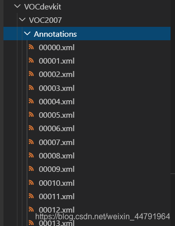
Before training, put the label file in the Annotation under the VOC2007 folder under the VOCdevkit folder.
Before training, put the picture file in JPEGImages under the VOC2007 folder under the VOCdevkit folder.

At this point, the placement of the data set has ended.
Second, the processing of data sets
After completing the arrangement of the data set, we need to process the data set in the next step. The purpose is to obtain 2007_train.txt and 2007_val.txt for training. We need to use voc_annotation.py in the root directory.
There are some parameters in voc_annotation.py that need to be set.
They are annotation_mode, classes_path, trainval_percent, train_percent, VOCdevkit_path, the first training can only modify classes_path
'''
annotation_mode用于指定该文件运行时计算的内容
annotation_mode为0代表整个标签处理过程,包括获得VOCdevkit/VOC2007/ImageSets里面的txt以及训练用的2007_train.txt、2007_val.txt
annotation_mode为1代表获得VOCdevkit/VOC2007/ImageSets里面的txt
annotation_mode为2代表获得训练用的2007_train.txt、2007_val.txt
'''
annotation_mode     = 0
'''
必须要修改,用于生成2007_train.txt、2007_val.txt的目标信息
与训练和预测所用的classes_path一致即可
如果生成的2007_train.txt里面没有目标信息
那么就是因为classes没有设定正确
仅在annotation_mode为0和2的时候有效
'''
classes_path        = 'model_data/voc_classes.txt'
'''
trainval_percent用于指定(训练集+验证集)与测试集的比例,默认情况下 (训练集+验证集):测试集 = 9:1
train_percent用于指定(训练集+验证集)中训练集与验证集的比例,默认情况下 训练集:验证集 = 9:1
仅在annotation_mode为0和1的时候有效
'''
trainval_percent    = 0.9
train_percent       = 0.9
'''
指向VOC数据集所在的文件夹
默认指向根目录下的VOC数据集
'''
VOCdevkit_path  = 'VOCdevkit'
classes_path is used to point to the txt corresponding to the detection category. Taking the voc dataset as an example, the txt we use is:

when training your own dataset, you can create a cls_classes.txt by yourself, and write the categories you need to distinguish in it.
3. Start network training
Through voc_annotation.py we have generated 2007_train.txt and 2007_val.txt, now we can start training.
There are many parameters for training. You can read the comments carefully after downloading the library. The most important part is still the classes_path in train.py.
classes_path is used to point to the txt corresponding to the detection category, this txt is the same as the txt in voc_annotation.py! Training your own data set must be modified!

After modifying the classes_path, you can run train.py to start training. After training for multiple epochs, the weights will be generated in the logs folder.
The functions of other parameters are as follows:
#---------------------------------#
#   Cuda    是否使用Cuda
#           没有GPU可以设置成False
#---------------------------------#
Cuda            = True
#---------------------------------------------------------------------#
#   distributed     用于指定是否使用单机多卡分布式运行
#                   终端指令仅支持Ubuntu。CUDA_VISIBLE_DEVICES用于在Ubuntu下指定显卡。
#                   Windows系统下默认使用DP模式调用所有显卡,不支持DDP。
#   DP模式:
#       设置            distributed = False
#       在终端中输入    CUDA_VISIBLE_DEVICES=0,1 python train.py
#   DDP模式:
#       设置            distributed = True
#       在终端中输入    CUDA_VISIBLE_DEVICES=0,1 python -m torch.distributed.launch --nproc_per_node=2 train.py
#---------------------------------------------------------------------#
distributed     = False
#---------------------------------------------------------------------#
#   fp16        是否使用混合精度训练
#               可减少约一半的显存、需要pytorch1.7.1以上
#---------------------------------------------------------------------#
fp16            = False
#---------------------------------------------------------------------#
#   classes_path    指向model_data下的txt,与自己训练的数据集相关
#                   训练前一定要修改classes_path,使其对应自己的数据集
#---------------------------------------------------------------------#
classes_path    = 'model_data/voc_classes.txt'
#----------------------------------------------------------------------------------------------------------------------------#
#   权值文件的下载请看README,可以通过网盘下载。模型的 预训练权重 对不同数据集是通用的,因为特征是通用的。
#   模型的 预训练权重 比较重要的部分是 主干特征提取网络的权值部分,用于进行特征提取。
#   预训练权重对于99%的情况都必须要用,不用的话主干部分的权值太过随机,特征提取效果不明显,网络训练的结果也不会好
#
#   如果训练过程中存在中断训练的操作,可以将model_path设置成logs文件夹下的权值文件,将已经训练了一部分的权值再次载入。
#   同时修改下方的 冻结阶段 或者 解冻阶段 的参数,来保证模型epoch的连续性。
#
#   当model_path = ''的时候不加载整个模型的权值。
#
#   此处使用的是整个模型的权重,因此是在train.py进行加载的,下面的pretrain不影响此处的权值加载。
#   如果想要让模型从主干的预训练权值开始训练,则设置model_path = '',下面的pretrain = True,此时仅加载主干。
#   如果想要让模型从0开始训练,则设置model_path = '',下面的pretrain = Fasle,Freeze_Train = Fasle,此时从0开始训练,且没有冻结主干的过程。
#
#   一般来讲,网络从0开始的训练效果会很差,因为权值太过随机,特征提取效果不明显,因此非常、非常、非常不建议大家从0开始训练!
#   如果一定要从0开始,可以了解imagenet数据集,首先训练分类模型,获得网络的主干部分权值,分类模型的 主干部分 和该模型通用,基于此进行训练。
#----------------------------------------------------------------------------------------------------------------------------#
model_path      = 'model_data/detr_resnet50_weights_coco.pth'
#------------------------------------------------------#
#   input_shape     输入的shape大小
#------------------------------------------------------#
input_shape     = [800, 800]
#---------------------------------------------#
#   vgg
#   resnet50
#---------------------------------------------#
backbone        = "resnet50"
#----------------------------------------------------------------------------------------------------------------------------#
#   pretrained      是否使用主干网络的预训练权重,此处使用的是主干的权重,因此是在模型构建的时候进行加载的。
#                   如果设置了model_path,则主干的权值无需加载,pretrained的值无意义。
#                   如果不设置model_path,pretrained = True,此时仅加载主干开始训练。
#                   如果不设置model_path,pretrained = False,Freeze_Train = Fasle,此时从0开始训练,且没有冻结主干的过程。
#----------------------------------------------------------------------------------------------------------------------------#
pretrained      = False

#----------------------------------------------------------------------------------------------------------------------------#
#   训练分为两个阶段,分别是冻结阶段和解冻阶段。设置冻结阶段是为了满足机器性能不足的同学的训练需求。
#   冻结训练需要的显存较小,显卡非常差的情况下,可设置Freeze_Epoch等于UnFreeze_Epoch,此时仅仅进行冻结训练。
#
#   在此提供若干参数设置建议,各位训练者根据自己的需求进行灵活调整:
#   (一)从整个模型的预训练权重开始训练:
#       AdamW:
#           Init_Epoch = 0,Freeze_Epoch = 50,UnFreeze_Epoch = 100,Freeze_Train = True,optimizer_type = 'adamw',Init_lr = 1e-4,weight_decay = 1e-4。(冻结)
#           Init_Epoch = 0,UnFreeze_Epoch = 100,Freeze_Train = False,optimizer_type = 'adamw',Init_lr = 1e-4,weight_decay = 1e-4。(不冻结)
#       其中:UnFreeze_Epoch可以在100-300之间调整。
#   (二)从主干网络的预训练权重开始训练:
#       AdamW:
#           Init_Epoch = 0,Freeze_Epoch = 50,UnFreeze_Epoch = 300,Freeze_Train = True,optimizer_type = 'adamw',Init_lr = 1e-4,weight_decay = 1e-4。(冻结)
#           Init_Epoch = 0,UnFreeze_Epoch = 300,Freeze_Train = False,optimizer_type = 'adamw',Init_lr = 1e-4,weight_decay = 1e-4。(不冻结)
#       其中:由于从主干网络的预训练权重开始训练,主干的权值不一定适合目标检测,需要更多的训练跳出局部最优解。
#             UnFreeze_Epoch可以在150-300之间调整,YOLOV5和YOLOX均推荐使用300。
#             Adam相较于SGD收敛的快一些。因此UnFreeze_Epoch理论上可以小一点,但依然推荐更多的Epoch。
#   (三)batch_size的设置:
#       在显卡能够接受的范围内,以大为好。显存不足与数据集大小无关,提示显存不足(OOM或者CUDA out of memory)请调小batch_size。
#       受到BatchNorm层影响,batch_size最小为2,不能为1。
#       正常情况下Freeze_batch_size建议为Unfreeze_batch_size的1-2倍。不建议设置的差距过大,因为关系到学习率的自动调整。
#----------------------------------------------------------------------------------------------------------------------------#
#------------------------------------------------------------------#
#   冻结阶段训练参数
#   此时模型的主干被冻结了,特征提取网络不发生改变
#   占用的显存较小,仅对网络进行微调
#   Init_Epoch          模型当前开始的训练世代,其值可以大于Freeze_Epoch,如设置:
#                       Init_Epoch = 60、Freeze_Epoch = 50、UnFreeze_Epoch = 100
#                       会跳过冻结阶段,直接从60代开始,并调整对应的学习率。
#                       (断点续练时使用)
#   Freeze_Epoch        模型冻结训练的Freeze_Epoch
#                       (当Freeze_Train=False时失效)
#   Freeze_batch_size   模型冻结训练的batch_size
#                       (当Freeze_Train=False时失效)
#------------------------------------------------------------------#
Init_Epoch          = 0
Freeze_Epoch        = 50
Freeze_batch_size   = 8
#------------------------------------------------------------------#
#   解冻阶段训练参数
#   此时模型的主干不被冻结了,特征提取网络会发生改变
#   占用的显存较大,网络所有的参数都会发生改变
#   UnFreeze_Epoch          模型总共训练的epoch
#                           SGD需要更长的时间收敛,因此设置较大的UnFreeze_Epoch
#                           Adam可以使用相对较小的UnFreeze_Epoch
#   Unfreeze_batch_size     模型在解冻后的batch_size
#------------------------------------------------------------------#
UnFreeze_Epoch      = 300
Unfreeze_batch_size = 4
#------------------------------------------------------------------#
#   Freeze_Train    是否进行冻结训练
#                   默认先冻结主干训练后解冻训练。
#------------------------------------------------------------------#
Freeze_Train        = True

#------------------------------------------------------------------#
#   其它训练参数:学习率、优化器、学习率下降有关
#------------------------------------------------------------------#
#------------------------------------------------------------------#
#   Init_lr         模型的最大学习率,在DETR中,Backbone的学习率为Transformer模块的0.1倍
#   Min_lr          模型的最小学习率,默认为最大学习率的0.01
#------------------------------------------------------------------#
Init_lr             = 1e-4
Min_lr              = Init_lr * 0.01
#------------------------------------------------------------------#
#   optimizer_type  使用到的优化器种类,可选的有adam、sgd
#                   当使用Adam优化器时建议设置  Init_lr=1e-4
#                   当使用AdamW优化器时建议设置  Init_lr=1e-4
#                   当使用SGD优化器时建议设置   Init_lr=1e-2
#   momentum        优化器内部使用到的momentum参数
#   weight_decay    权值衰减,可防止过拟合
#                   adam会导致weight_decay错误,使用adam时建议设置为0。
#------------------------------------------------------------------#
optimizer_type      = "adamw"
momentum            = 0.9
weight_decay        = 1e-4
#------------------------------------------------------------------#
#   lr_decay_type   使用到的学习率下降方式,可选的有step、cos
#------------------------------------------------------------------#
lr_decay_type       = "cos"
#------------------------------------------------------------------#
#   save_period     多少个epoch保存一次权值
#------------------------------------------------------------------#
save_period         = 10
#------------------------------------------------------------------#
#   save_dir        权值与日志文件保存的文件夹
#------------------------------------------------------------------#
save_dir            = 'logs'
#------------------------------------------------------------------#
#   eval_flag       是否在训练时进行评估,评估对象为验证集
#                   安装pycocotools库后,评估体验更佳。
#   eval_period     代表多少个epoch评估一次,不建议频繁的评估
#                   评估需要消耗较多的时间,频繁评估会导致训练非常慢
#   此处获得的mAP会与get_map.py获得的会有所不同,原因有二:
#   (一)此处获得的mAP为验证集的mAP。
#   (二)此处设置评估参数较为保守,目的是加快评估速度。
#------------------------------------------------------------------#
eval_flag           = True
eval_period         = 10
#------------------------------------------------------------------#
#   官方提示为TODO this is a hack
#   稳定性未知,默认为不开启
#------------------------------------------------------------------#
aux_loss            = False
#------------------------------------------------------------------#
#   num_workers     用于设置是否使用多线程读取数据
#                   开启后会加快数据读取速度,但是会占用更多内存
#                   内存较小的电脑可以设置为2或者0
#------------------------------------------------------------------#
num_workers         = 4

#----------------------------------------------------#
#   获得图片路径和标签
#----------------------------------------------------#
train_annotation_path   = '2007_train.txt'
val_annotation_path     = '2007_val.txt'
4. Prediction of training results
Two files are required for training result prediction, namely detr.py and predict.py.
We first need to modify model_path and classes_path in detr.py, these two parameters must be modified.
model_path points to the trained weight file in the logs folder.
classes_path points to the txt corresponding to the detection category.

After completing the modification, you can run predict.py for detection. After running, enter the image path to detect.