[Eating the book together] "Machine Learning" Chapter 8 Integrated Learning

Chapter 8 Integrated Learning

8.1 Individuals and Ensembles

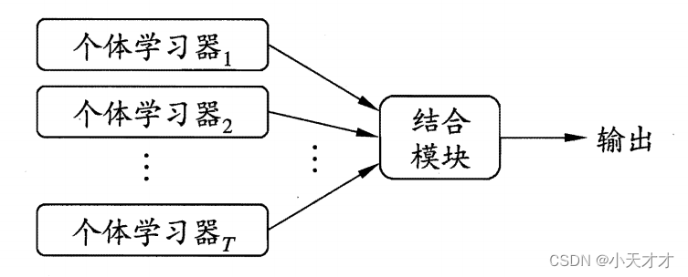
  Integrated learning completes learning tasks by building and combining multiple learners, sometimes called multi-classifier systems, committee-based learning, etc. The following is the general structure of integrated learning: first generate a set of "individual learners", and then Combine them with some strategy. If the integration only contains the same type of individual learners, this integration is called a homogeneous integration, and the individual learners inside are also called "base learners"; if it contains different types of individual learners, this integration It is called heterogeneous integration, and the individual learners in it are also called "component learners".

  In general experience, if you mix individual learners that are not equal to good or bad, then usually the result will be better than the worst and worse than the best. To obtain a good integration, the individual learner should be " Good and different", that is, individual learners must have a certain "accuracy", and there must be "diversity", which means that there are differences between learners, as shown below.

  According to the generation method of individual learners, the current ensemble learning methods can be roughly divided into two categories, that is, there are strong dependencies between individual learners, serialization methods that must be generated serially, and there is no strong dependency between individual learners. , A parallel method that can be generated at the same time; the representative of the former is Boosting, and the representative of the latter is Bagging and "random forest".

8.2 Boosting

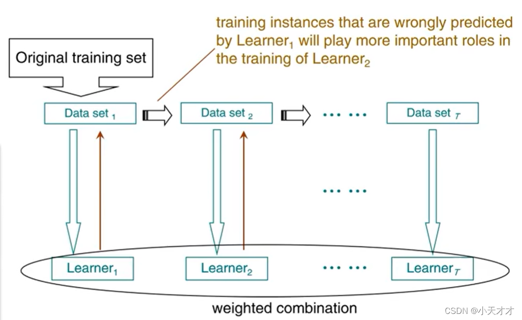
  Boosting is an algorithm that can upgrade a weak learner to a strong learner: first train a base learner from the initial training set, and then adjust the distribution of training samples according to the performance of the base learner, so that the previous base learner Wrong training samples receive more attention in the follow-up, and then the next base learner is trained based on the adjusted sample distribution; this is repeated until the number of base learners reaches the value TT specified in $T$ , and eventually this$T$ base learners are weighted and combined as follows:

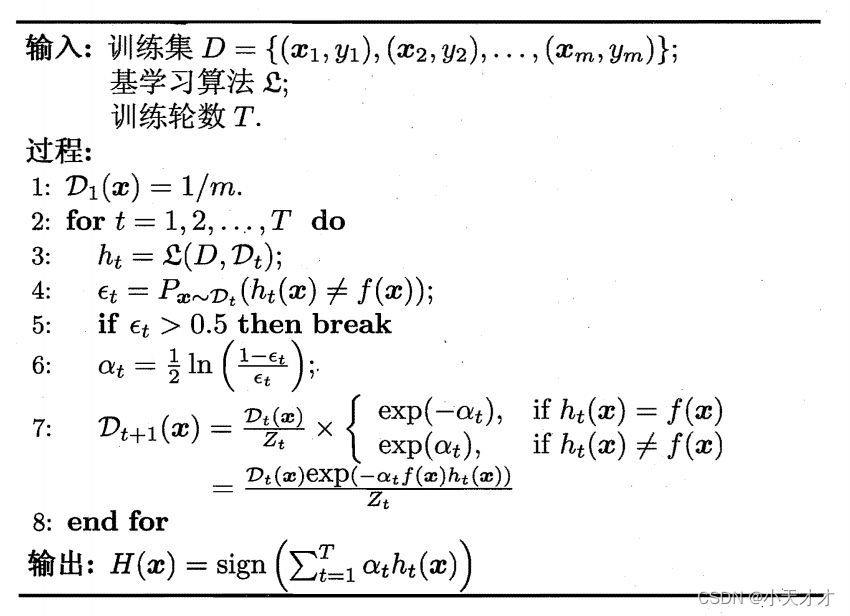
  The most famous representative of the Boosting algorithm is AdaBoost, as shown below

  The Boosting algorithm requires the base learner to be able to learn a specific data distribution, which can be achieved through the "reweighting method", that is, in each round of the training process, a weight is assigned to each training sample according to the sample distribution. For learning algorithms that cannot accept weighted samples, it can be realized through the "resampling method", that is, in each round of learning, the training set is re-sampled according to the sample distribution, and then the sample set obtained by resampling is used to compare the base The learner is trained. It should be noted that the Boosting algorithm checks whether the currently generated base learner meets the basic conditions in each round of training.

  The following is an example of the AdaBoost algorithm on the watermelon dataset. The thick black line in the figure is the classification boundary of the integration, and the thin black line is the classification boundary of the base learner.

8.3 Bagging and Random Forest

  If you want to obtain an ensemble with strong generalization ability, the individual learners in the ensemble should be as independent as possible. Although "independence" cannot be achieved in real-world tasks, you can try to make the base learners have as large a difference as possible. A possible approach is to sample the training samples to generate several different subsets, and then train a base learner from each data subset.

  Bagging is based on self-service sampling method, for a given including $For\; a\; data\; set\; of\; m$ samples, first randomly take a sample and put it into the sampling set, and then put the sample back into the initial data set, so that the sample may still be selected in the next sampling, so that after$m$ random sampling operations, you can$A\; sampling\; set\; of\; m$ samples, and finally TTcan also be sampled$T$ includes$A\; sample\; set\; of\; m$ training samples, and then a base learner is trained based on each sample set, and then these base learners are combined. Bagging typically uses simple voting for classification tasks and simple averaging for regression tasks when combining predicted outputs. Below is an example of running the Bagging algorithm on the watermelon dataset.

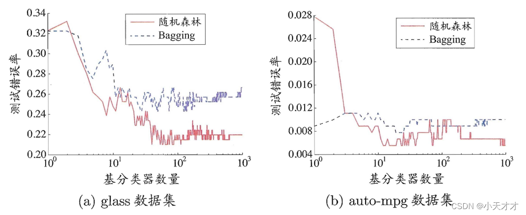
  Random Forest (Random Forest) is an extended variant of Bagging. On the basis of constructing Bagging ensemble based on decision tree-based learner, it further introduces random attribute selection in the training process of decision tree. Specifically, when the traditional decision tree selects the partition attribute, it is the attribute set of the current node (assuming $d$ attributes) to select an optimal attribute; and in random forest, for each node of the base decision tree, first randomly select a node containing kkfrom the attribute set of the node$A\; subset\; of\; k$ attributes, and then select an optimal attribute from this subset for division. In general, the recommended value$k=lo{g}_{2}d$。

• The diversity of base learners in random forest comes not only from sample perturbation, but also from attribute perturbation, which makes the generalization performance of the final ensemble further improved by increasing the difference between individual learners.
• The training efficiency of random forest is better than that of Bagging, because in the process of constructing individual decision trees, Bagging uses a "deterministic" decision tree. A "random" decision tree only needs to examine a subset.

8.4 Combining Strategies

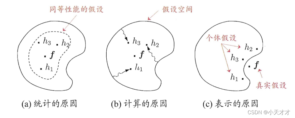
  Combining learners may benefit in three ways:

• From a statistical point of view, since the hypothesis space of the learning task is often large, there may be multiple hypotheses that can achieve the same performance on the training set. At this time, if a single learner is used, the generalization performance may be poor due to misselection. Multiple learners reduce this risk.
• From a computational point of view, learning algorithms tend to fall into local minima, and the generalization performance corresponding to some local minima may be poor, and combining multiple runs can reduce the chance of falling into bad local minima. risks of.
• From the perspective of representation, the real hypothesis of some learning tasks may not be in the hypothesis space considered by the current learning algorithm. At this time, if a single learner is used, it will definitely be invalid. However, by combining multiple learners, due to the corresponding hypothesis space With some dilation, it is possible to learn better approximations.

  The commonly used combination strategies are as follows:

(1) Average method

  The weighted average method should be used when the performance of individual learners is quite different, and the simple average method should be used when the performance of individual learners is similar.

(2) Voting method

• Absolute majority voting method: If a mark gets more than half of the votes, the mark is predicted, otherwise the prediction is rejected.
• Relative majority voting method: predict the mark with the most votes, if there are multiple marks with the highest votes at the same time, one of them will be randomly selected.
• Weighted voting method: Similar to the weighted average method, a weight is set for each voting party.

(3) Learning method

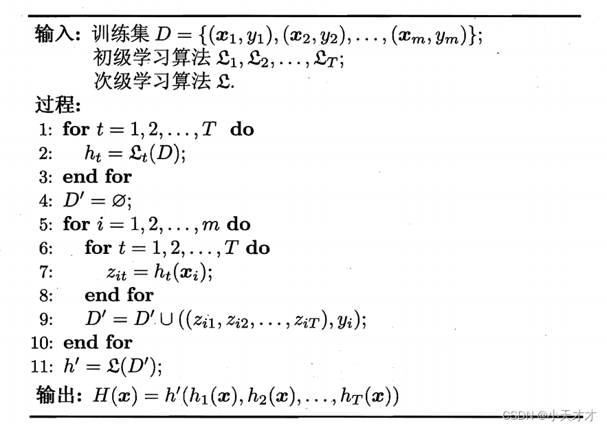
  When there is a lot of training data, a more powerful combination strategy is to use the "learning method", that is, to combine through another learner, such as the Stacking algorithm. Here we call the individual learner a primary learner, which is used to combine The learner is called a secondary learner or meta-learner.

  The Stacking algorithm is an integrated learning method that uses multiple different base learners to predict data, and then inputs the prediction results as new features into a meta-learner to obtain the final classification or regression results. The Stacking algorithm can take advantage of different base learners to improve generalization performance, and can also use cross-validation or leave-one-out method to prevent overfitting.

8.5 Diversity

(1) Error-difference decomposition

  Error-divergence decomposition is a method to decompose the generalization error of ensemble learning into the error of individual learners and divergence, where error represents the average generalization error of individual learners, and divergence represents the inconsistency or diversity among individual learners . The formula for error-difference decomposition is as follows:
$$E=\bar{E}-\bar{A}$$
  Among them,$E$ is the integrated generalization error,$\bar{E}$ is the average generalization error of individual learners,$\bar{A}$ is the average divergence of individual learners. This formula shows that the higher the accuracy and diversity of individual learners, the better the ensemble. Error-divergence decomposition is only applicable to regression problems, and it is difficult to generalize to classification problems. The error-divergence decomposition is based on the derivation of the squared error, which is a common loss function for regression problems. For classification problems, squared error is not necessarily an appropriate loss function because it does not reflect the degree of misclassification very well. Therefore, the error-divergence decomposition is difficult to directly generalize to classification learning tasks.

(2) Diversity measure

• Unsuitable measure

$$di{s}_{ij}=\frac{b+c}{m}$$

  $di{s}_{ij}$The value range is $[0,1]$ , the greater the value, the greater the diversity.

• correlation coefficient

$$r_{ij}=\frac{ad-bc}{\sqrt{(a+b)(a+c)(c+d)(b+d)}}$$

  $r_{ij}$The range of values ​​is $[-1,1]$，Wakahi$h_i$with $h_j$irrelevant, the value is 0; if $h_i$with $h_j$The value is positive if there is a positive correlation, and negative otherwise.

• $Q$ - statistic

$$Q_{ij}=\frac{ad-bc}{ad+bc}$$

  $Q_{ij}$Correlation coefficient $r_{ij}$have the same sign, and $\left|Q_{ij}\right|⩾\left|{\rho }_{ij}\right|$。

• $\kappa$ -statistic

$$\begin{array}{rl}& K=\frac{p_1-p_2}{1-p_2}\\ & p_1=\frac{a+d}{m}\\ & p_2=\frac{(a+b)(a+c)+(c+d)(b+d)}{m^2}\end{array}$$

  Among them, $p_1$is the probability that two classifiers agree, $p_2$is the probability that two classifiers agree by chance, if the classifier $h_i$with $h_j$in $D$ is completely consistent, then$K=1$ ; if they agree only by chance, then$K=0$ .$\kappa$ is usually non-negative, only at$h_i$with $h_j$Negative values ​​are taken where the probability of agreement is even lower than chance.

(3) Diversity measure selection

• Disagreement measure refers to the probability that individual classifiers give different classification results for the same sample. A larger discrepancy measure indicates greater differences between individual classifiers.
• The correlation coefficient refers to the degree of linear correlation between individual classifiers. The smaller the correlation coefficient, the larger the difference between individual classifiers.
• Q-statistics refers to the difference between the probability that two classifiers are both correct or both wrong on the same sample and the probability that only one classifier is correct. The smaller the Q statistic, the larger the difference between individual classifiers.
• $\kappa$ -statistic ($\kappa$ -statistic) is the difference between the probability that two classifiers agree on the same sample and the probability that they agree by chance. $The\; smaller\; the\; \kappa$ statistic, the larger the difference between individual classifiers.

(4) Enhanced diversity

• Data sample perturbation: Given an initial data set, different data subsets can be generated from it, and then different individual learners can be trained using different data subsets.
• Input attribute perturbation: Extract several attribute subsets from the initial attribute set, and then train a base learner based on each attribute subset.
• Output representation perturbation: Slightly change the class label of the training sample, or convert the output representation, or decompose the original task into multiple subtasks that can be solved simultaneously.
  Generate different data subsets, and then use different data subsets to train different individual learners.
• Algorithm parameter disturbance: By randomly setting different parameters, individual learners with large differences are generated.