
Recommendation: Use NSDT Designer to quickly build programmable 3D scenes.
Determining what lies below the ground and effectively mapping it out is one of the first and most important parts when designing any type of engineered structure. Subsurface modeling comes with a large margin of error, as even the most advanced subsurface survey methods we use today cannot fully map soil, rock, water levels, etc. over larger areas. Whether you're using boreholes (SPT or CPT), seismic refraction, or some other method, you'll eventually have to do a lot of interpolation to build your subsurface model.
Software such as Bentley's GINT is well suited to creating 2D and 3D soil profiles, the accuracy of which is really only limited by the data provided and the experience of the engineer. These subsurface models can also be created using Python, and while it's not as simple as GINT, it gives us more freedom to manipulate our models as we see fit. Once you get the hang of it, you can generate a good soil profile faster than some software, and definitely faster than drawing it in CAD.
Below is a tutorial on how to create a 3D model of the subsurface using Python, focusing on the open source geological modeling library GemPy. It is capable of constructing complex 3D geological models of folded structures, fault networks and unconformities.
1. Install and configure GemPy
GemPy can be installed with the following command:
pip install gempy
We need data from the project site and subsurface surveys, in CSV format, because we'll use pandas to convert them into a data frame:
- Surface_points → in situ measured surface elevations for the area (x,y,z)
- Orientations → Assign stratigraphic values to surface points (Gx, Gy, Gz or Azimuth). Essentially, it is the angle associated with a surface point representing a fault through the layer
- Grid → model size (number of columns x number of rows x number of layers)
- Surfaces → Soil/Rock Layers
- Series → group surfaces and faults into separate series
- Faults → Location and information of faults to be modeled (must be inserted separately)
For this tutorial, we will call the CSV file containing these 6 parameters "MyProject.csv".
Modeling with GemPy requires first importing the necessary packages:
from pyvista import set_plot_theme

%matplotlib inline

import gempy as gp
import numpy as np
import pandas as pd
import matplotlib.pyplot as plt
2. Use GemPy to load geological data
First, we need to extract the data from the CSV file containing site information into a data frame and create a model using GemPy.
geo_model = gp.create_model('MyProject')

# Importing the data from CSV-files and setting our boundaries
gp.init_data(geo_model, [0, 2000., 0, 2000., 0, 2000.], [100, 100, 100],
             path_o= "MyProject_model_orientations.csv",
             path_i= " MyProject_model_points.csv",)
This will generate the address model, our data as 100 rows x 100 columns x 100 layers, spanning a volume of 2km x 2km x 2km, our 'resolution' and 'grid size' respectively. The bigger you get, the longer it takes to run the model. The model takes in both the Surface_point data (path_i) and the direction (path_o) that will be used for interpolation and generates our 2D and 3D plots.
Using .surface() we see that the geo_model made with the "MyProject" data has 5 such surfaces where the Basement is automatically generated and acts as a lower bound:
geo_model.surfaces
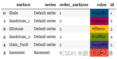
Surface layers need to be separated into two separate classification series, stratigraphic surface layers (Strat_Series) and faults (Fault_Series). GemPy is a bit picky when it comes to the order of these surfaces. Faults always need to be moved to the top, independently of each other, their order determines which goes through the surface first (tectonic relationship). The order of the Strat_Series surface should represent the real world location we are modeling, the basement is always at the bottom. We can achieve this by:
gp.map_stack_to_surfaces(geo_model,
                         {"Fault_Series": 'Main_Fault',
                          "Strat_Series": ('Sandstone_2',
                          'Siltstone', 'Shale', 'Sandstone_1',
                          'basement')},
                          remove_unused_series=True)
geo_model.surfaces

All we've done is put a Fault_Series on top, but now that the model surfaces are ordered, Gempy should handle them without a problem.
3. Use GemPy to visualize initial data
We can create 2D and 3D plots of the initial data for visualization, which also shows us the interface and orientation.
# 2-D
gp.plotta(geo_data,
direction='y')
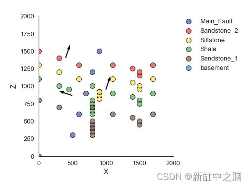
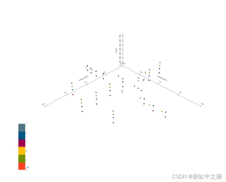
# 3-D
gp.plot_3d(geo_model,
plotter_type='basic')
4. Use GemPy to interpolate geological data
The plot above doesn't look like much, especially in 3D. We want to fill this grid, basically make it a solid 2km x 2km x 2 km block, as if you'd ripped out a huge chunk of the earth to examine it. To do this, we will fill the plot by interpolating the current data.
GemPy uses a method called Kriging for interpolation, also known as Gaussian process regression, which is a covariance-governed method that provides optimal linear unbiased predictions at unsampled locations. We insert data like this:
interpol_data = gp.InterpolatorData(geo_data, output='geology',
                                    compile_theano=True,
                                    theano_optimizer='fast_compile')
The kriging parameters can be changed if desired, but I personally don't mess with them.
gp.get_data(geo_model, 'kriging')

5. Use GemPy to calculate geological models
After interpolation, we can use GemPy to create our model:
gp.compute_model(interpol_data)
The resulting model will generate two arrays, one for the geological surface and one for the faults (Faults) that pass through the surface.
interpol_data.geo_data_res.get_formations()
The result is as follows:
Surfaces Array: [Main_Fault, Sandstone_2, Siltstone, Shale, Sandstone_1]

Fault Array:(5, object) [Main_Fault, Sandstone_2, Siltstone, Shale, Sandstone_1]
These two arrays also have 2 sub-arrays as solutions for the block model.
6. Visualize geological models with GemPy
Geological models generated by GemPy can be visualized in 2D or 3D, and topographic maps can be added.
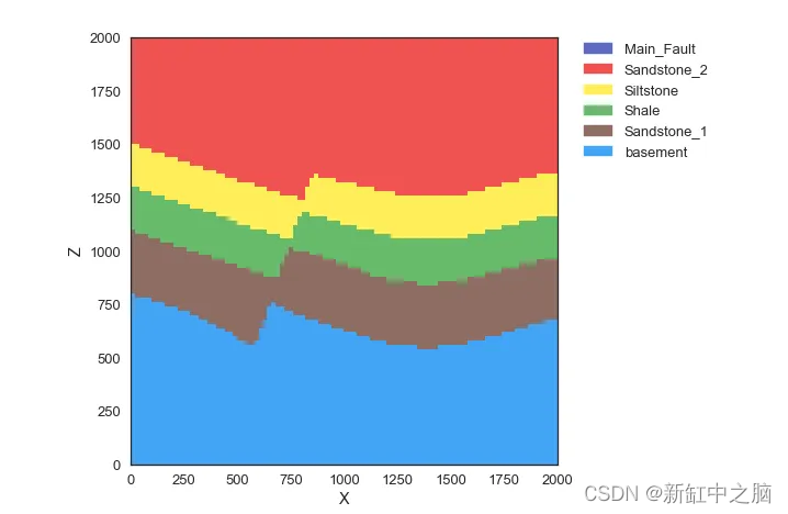
6.1 2D visualization
Using Matplotlib, we can plot the model we just generated and create the soil profile we've been after. The code below will basically take a 2km³ block (represented by a 100 row x 100 column x 100 layer grid) and slice it at the y=50 mark, giving us a cross section in the middle of the model.
gp.plotting.plot_section(geo_data,
                         gp.compute_model(interpol_data)[0],
                         cell_number=50, direction='y',
                         plot_data=False)
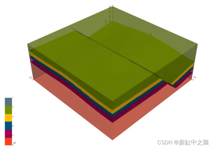
6.2 3D visualization
We can visualize our models in 3d using VTK, an open source software system for 3D computer graphics, image processing, and scientific visualization. It's already integrated into GemPy, so there's no need to import anything new.
We first need to get the vertices and triangulation from our surface and the function get_surface. We can then use these to plot our 3-D models:
ver, sim = gp.get_surfaces(interpol_data, original_scale=True)

gp.plotting.plot_surfaces_3D(geo_data, ver, sim,
                             plotter_type='basic')
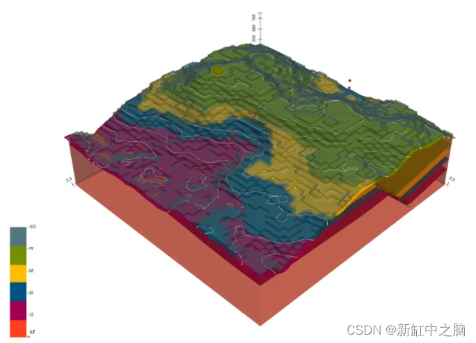
6.3 Add terrain map
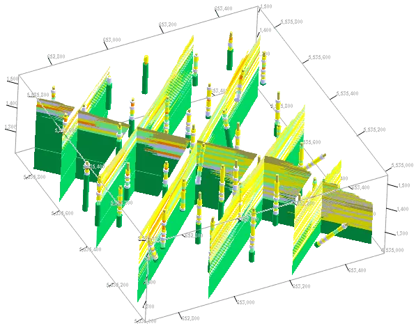
Adding terrain always makes a model look better than just some blocks. Terrains are highly customizable as you can use real world raster images, create your own surface overlays, color changes based on elevation, and many more options. We'll add a terrain map based on depth and layer color.
geo_model.set_topography(d_z=(1000, 2000))

gp.plot_3d(interpol_data, plotter_type='basic',
                 show_topography=True, show_surfaces=True,
                 show_lith=True, image=False)
7. Conclusion
This tutorial is for creating a basic geological 3D model from which you can extract 2D cross-sectional soil profiles and use them for design. It definitely needs to incorporate things like groundwater elevation, soil/rock parameters, etc. to make each layer really useful. In the end, we end up with a highly interactive model from which information can be easily extracted.
Original link: GemPy geological modeling practice - BimAnt