I have completed six blogs about time series before , readers who have not read them, please read them first:

6. Data Analysis of Time Series (6): Exponential Smoothing Forecasting Method

Data Stationarity

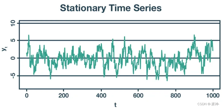
Data stationarity means that the statistical properties of time series such as mean, variance, and covariance do not change with time. In other words, the mean, variance, and covariance of a time series remain constant over time.

How to Assess Stationarity of Data: Visual Evaluation

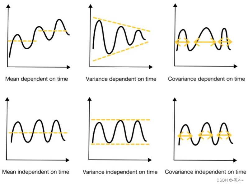
If the time series data has three characteristics of constant mean, variance and covariance at the same time, then we can assume that the data is stationary, otherwise the data is non-stationary. Therefore, we can observe the changing law of the data through a simple visual method, so that we can judge whether the data is stable:

Simple calculations to identify stationarity in data

We can roughly divide time series data into two halves: the first half and the second half. And compare the mean, amplitude, and period length of the first half and the second half. Here the amplitude corresponds to the variance, and the period length corresponds to the covariance.

Constant mean: the mean of the first half and the second half of the data are similar (no need to be absolutely equal)
Constant variance: the first and second halves of the data have similar amplitudes (no need to be absolutely equal)
Constant covariance: the period lengths of the first and second halves of the data are similar (do not need to be absolutely equal)

If the time series data has the three characteristics of constant mean, constant variance and constant covariance, then we can assume that the data is stationary, otherwise the data is not stationary.

Statistical tests to assess stationarity

Strict statistical tests to assess the stationarity of data are also known as unit root tests, and a single root is a random trend known as a "random walk with drift". Since randomness cannot be predicted, this means:

There is a unit root: non-stationary (unpredictable)
no unit root: stationary

To assess stationarity using a unit root test requires the use of a hypothesis test:

Null hypothesis (H0): The time series is stationary (there is no single root)
Alternative hypothesis (Alternative hypothesis, H1): the time series is not stationary (there is a unit root)

Note that the specific hypothetical content of H0 and H1 here is not necessarily subject to the above content, or it may be just the opposite, and the hypothetical content must be determined by specific testing methods.

Then, whether to reject the null hypothesis will be evaluated based on the statistical calculation results, if H0 is rejected, it means the acceptance of H1, and vice versa.

p-value method:
If p-value > 0.05, the null hypothesis cannot be rejected.
The null hypothesis was rejected if the p-value was ≤ 0.05.

Critical value method:
If the test statistic is less extreme than the critical value, the null hypothesis cannot be rejected.
The null hypothesis is rejected if the test statistic is more extreme than the critical value.

NOTE: The critical value method should be used when the p-value is close to significant (for example, around 0.05).

Commonly used single root inspection methods

1. Augmented Dicky Fuller Test (ADF test)

The hypothesis for the Augmented Dickey-Fuller (ADF) test is:

Null Hypothesis (H0): The time series is non-stationary because there is a unit root (if p-value > 0.05)
Alternative hypothesis (H1): The time series is stationary because there is no unit root (if p-value ≤ 0.05)

In Python, we can use the adfuller method of the statsmodels package to implement the ADF test. However, in order to test the validity of the single root test results, we have prepared two sets of data in advance, one is the passenger number data of airlines over the years, and the other is white noise data. The passenger data here has an obvious trend, so it is non-stationary , while the white noise data is stationary.

import pandas as pd
import numpy as np
import matplotlib.pyplot as plt
plt.style.use('ggplot')
plt.rc("figure", figsize=(10,4))

#非平稳的航空乘客数据
df=pd.read_csv('passengers.csv').set_index('Period')
df.plot();

# 平稳的白噪声序列
np.random.seed(10)
y= np.random.normal(loc=0,scale=1,size=500)
white_noise = pd.Series(y)
white_noise.plot();

Next, we use adf to test the stationarity of these two data respectively.

from statsmodels.tsa.stattools import adfuller

#航空公司乘客数据adf检验
result = adfuller(df["passengers"].values)

print('ADF Statistics: %f' % result[0])
print('p-value: %f' % result[1])
print('Critical values:')
for key, value in result[4].items():
    print('\t%s: %.3f' % (key, value))

print(f'Result: The series is {"not " if result[1] > 0.05 else ""}stationary')

Judgment criteria:

If P-value <=0.05 and test statistic<1% of the critical value (Critical values) then reject the null hypothesis.
Accept the null hypothesis if P-value > 0.05 or test statistic > 1% of critical values.

Here our P-value is 0.99 > 0.05 so accept the null hypothesis that the data is non-stationary. (the null hypothesis of adf is that the data is non-stationary).

#白噪声的adf建议结果
result = adfuller(white_noise.values)
print('ADF Statistics: %f' % result[0])
print('p-value: %f' % result[1])
print('Critical values:')
for key, value in result[4].items():
    print('\t%s: %.3f' % (key, value))
print(f'Result: The series is {"not " if result[1] > 0.05 else ""}stationary')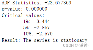

Here the pvale value is 0.0<0.05 and the test statistic value is -23.677<1% critical value -3.443, so reject H0 and accept H1, that is, the data is stable.

2. Kwiatkowski-Phillips-Schmidt-Shin Test (KPSS test)

KPSS is a test method used to calculate the null hypothesis that the data is horizontal or trend stationary.

The hypothesis of the KPSS test is:

Null Hypothesis (H0): The time series is stationary because there is no unit root (if p-value > 0.05)
Alternative Hypothesis (H1): The time series is non-stationary because there is a unit root (if p-value ≤ 0.05)

Note: KPSS test and ADF test their assumptions are just opposite.

In Python, we can use the kpss method of the statsmodels package to implement the KPSS test. There is a parameter regression in kpss, because the airline passenger data has an obvious trend and seems to be stable, so regression must be set to "ct"

from statsmodels.tsa.stattools import kpss
# 检验航空乘客数据
statistic, p_value, n_lags, critical_values = kpss(df["passengers"].values,
                                                   regression = "ct");
print(f'KPSS Statistic: {statistic}')
print(f'p-value: {p_value}')
# print(f'num lags: {n_lags}')
print('Critial Values:')
for key, value in critical_values.items():
    print(f'   {key} : {value}')
print(f'Result: The series is {"not " if p_value < 0.05 else ""}stationary')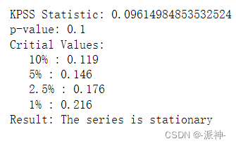

Judgment criteria:

1. If P-value <=0.05 and test statistic>Critical values, reject the null hypothesis.
2. If P-value > 0.05 or test statistic < critical values (Critical values) then accept the null hypothesis.

Here our P-value is 0.1 > 0.05 so accept the null hypothesis that the data is stationary.

#检验白噪声
statistic, p_value, n_lags, critical_values = kpss(white_noise.values)
print(f'KPSS Statistic: {statistic}')
print(f'p-value: {p_value}')
print(f'num lags: {n_lags}')
print('Critial Values:')
for key, value in critical_values.items():
    print(f'   {key} : {value}')
print(f'Result: The series is {"not " if p_value < 0.05 else ""}stationary')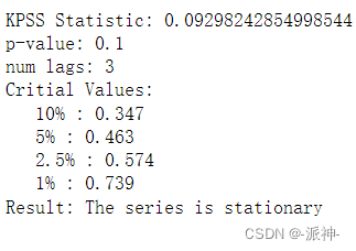

Here the P-value of white noise is 0.1 > 0.05 so accept the null hypothesis that the data is stationary.

Problems with the single root test

Different single root test methods such as adf, kpss, etc. sometimes give diametrically opposite conclusions, which can confuse people. In order to ensure the correctness of the test results, we must use two or more methods to test at the same time, as follows It is the situation that will be encountered when two methods are used for inspection:

Case 1: The conclusions drawn by both tests are stationary, then the data is stationary.
Case 2: The conclusions drawn by both tests are non-stationary, then the data is non-stationary.
Situation 3: ADF draws a non-stationary conclusion, and KPSS draws a stable conclusion, then the data is trend-stable.
Situation 4: ADF draws a stable conclusion, and KPSS draws a non-stationary conclusion, then the data is differentially stationary.

How to deal with non-stationary data

When our time series time is non-stationary, then we can make the data smooth by the following methods:

difference
Detrending by model fitting
logarithmic transformation

1. Difference

Differencing calculates the difference between two consecutive observations. It stabilizes the mean of the time series, reducing the trend. Let's use Tesla's stock data to implement the difference operation:

#加载特斯拉股票数据
df= pd.read_csv('./data/tsla.csv')
df.date=pd.to_datetime(df.date)

# 对特斯拉股票数据进行差分处理
df['diff_Close']= df['Close'].diff()

#绘图
fig, axs = plt.subplots(2, 1,figsize=(10,8))
axs[0].plot(df.date,df.Close)
axs[0].set_title('Tsla Stock Price')
axs[1].plot(df.date,df.diff_Close)
axs[1].set_title('differencing Tsla Stock Price')
plt.show();

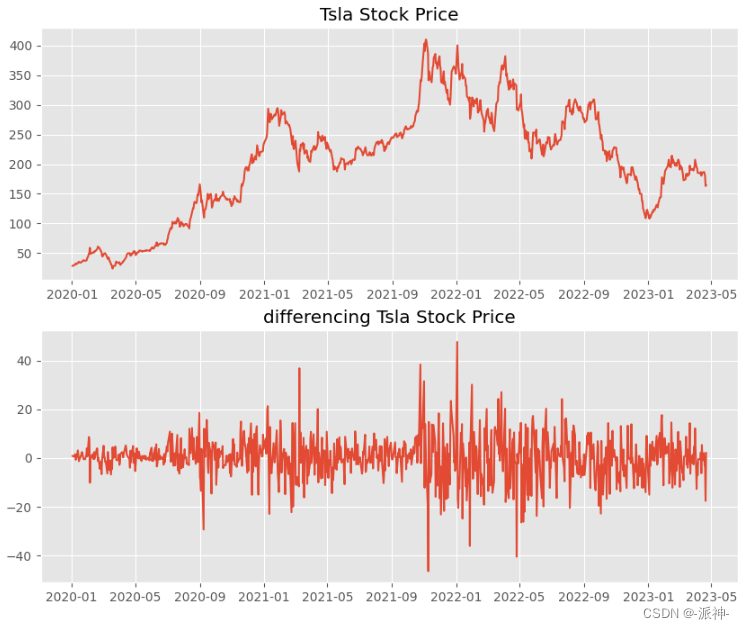
After performing the first-order difference operation on the Tesla stock data, we get a sequence similar to white noise, which is approximately stationary. Sometimes if the result of the first-order difference is still not stable, then the second-order difference operation can also be performed, but generally no more than the second-order difference is performed.

2. Detrend by model fitting

One way to remove trend from a non-stationary time series is to fit a simple model such as linear regression to the data, and then model the residuals from that fit.

from sklearn.linear_model import LinearRegression

#非平稳的航空乘客数据
df=pd.read_csv('passengers.csv')
df.Period=pd.to_datetime(df.Period)

# 训练线下回归模型 
X = [i for i in range(0, len(df))]
X = np.reshape(X, (len(X), 1))
y = df["passengers"].values
model = LinearRegression()
model.fit(X, y)

# 计算趋势
trend = model.predict(X)

# 去除趋势
df["detrend"] = df["passengers"].values - trend

#绘图
fig, axs = plt.subplots(2, 1,figsize=(10,8))
axs[0].plot(df.Period,df.passengers)
axs[0].set_title('passengers')
axs[1].plot(df.Period,df.detrend)
axs[1].set_title('detrend passengers')
plt.show();

The method of detrending can stabilize the mean value of the data, but the stability of the mean value does not mean that the data is stable. The above air passenger data regrets after the detrend operation. Although the mean value is stable, the variance is still unstable. Can the variance be made Also become stable?

3. Log transformation

Logarithmic transformation can make the variance of time series data more stable. After the above-mentioned airline passenger data is detrended, the mean value becomes stable, but the variance is still unstable. Therefore, we need to do logarithmic transformation to make the variance change Be stable.

df=pd.read_csv('passengers.csv')
df.Period=pd.to_datetime(df.Period)
#对数变换
df['log_passengers'] = np.log(df['passengers'].values)

# 训练线下回归模型 
X = [i for i in range(0, len(df))]
X = np.reshape(X, (len(X), 1))
y = df["log_passengers"].values
model = LinearRegression()
model.fit(X, y)

# 计算趋势
trend = model.predict(X)

# 去除趋势
df["detrend_log_passengers"] = df["log_passengers"].values - trend

#绘图
fig, axs = plt.subplots(3, 1,figsize=(10,10))
axs[0].plot(df.Period,df.passengers)
axs[0].set_title('passengers')
axs[1].plot(df.Period,df.log_passengers)
axs[1].set_title('log passengers')

axs[2].plot(df.Period,df.detrend_log_passengers)
axs[2].set_title('detrend log passengers')
plt.show();

After the above data undergoes logarithmic transformation and detrending operation, the data becomes stable in mean and variance, so it is an ideal result.

Summarize

In time series forecasting, when time series data have constant statistical properties (mean, variance, and covariance) and these statistical properties are independent of time, then the data are said to be stationary. Due to the constant statistical properties, stationary time series are easier to model than non-stationary time series. Therefore, many time series forecasting models assume that the data are stationary.

Stationarity can be checked by visual evaluation or statistical methods. Statistical methods check whether there is a unit root in the data. The two most commonly used single root tests are ADF and KPSS. We can call them in Python's third-party library statsmodels.tsa.stattools.

If the time series is non-stationary, you can try to make it stationary by differencing, log-transforming, or detrending.

References

stationarity_detrending_adf_kpss

statmodels.tsa.stattools.adfuller

statsmodels.tsa.stattools.kpss

Data Analysis of Time Series (7): Data Stationarity