Batch and Momentum

Momentum method

Momentum is momentum, that is, the loss function will not stop directly when it reaches the critical point of the gradient, and can directly rush through the critical point with the previous (larger) gradient.

In the real physical world, it will not be stuck by saddle point or local minima. A technique similar to this is the momentum method.

Vanilla Gradient Descent general gradient descent

vanilla grass jelly

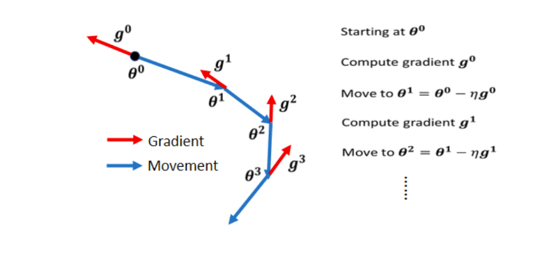
At the initial point, determine a g0, and move in the opposite direction of this at the same time. To update the parameter in the opposite direction of the gradient

$\theta ^{1}=\theta ^{0}-\eta g^{0}$

Gradient Descent + Momenturn

After using Momentum, every time you update the parameters, instead of going to the opposite direction of the gradient, you use the opposite direction of the gradient, plus the direction of the previous step, because they are all vectors, and the result of adding the two

The initial parameter $\theta ^{0}$ , at this time, the parameter of the update in the previous step is $m^{0}=0$ .

Next, calculate the direction of the Gradient $\Theta ^{0}$ at the place $g^{0}$ , and the previous step is exactly 0, so the direction of the update does not change. But it has changed since the second one, but here $\lambda \and$ are all parameters that need to be set by yourself. The second m is the joint action of the first m and the first g

g1 tells us that Gradient tells us to go in the opposite direction of red , but we don't just listen to Gradient, after adding Momentum, we don't just adjust our parameters according to the opposite direction of Gradient, we will also look at the previous time Direction of Update
1. If the previous time said to go $m^{1}$ in the direction of blue and blue dotted lines
2. Gradient said to go in the direction opposite to red
3. Add the two together and take a compromise between the two, that is Go in the direction of blue $m^{2}$ , so we move m2 and go to the place of θ2

Next, we repeat the same process. At this position, we calculate the Gradient, but we don’t just walk in the opposite direction based on the Gradient. We see how to go in the previous step. The previous step goes in this direction, and in the direction of the blue dotted line, we put The blue dotted line plus the red dotted line, the direction indicated by the previous step and the direction indicated by Gradient are used as the direction we want to move in the next step

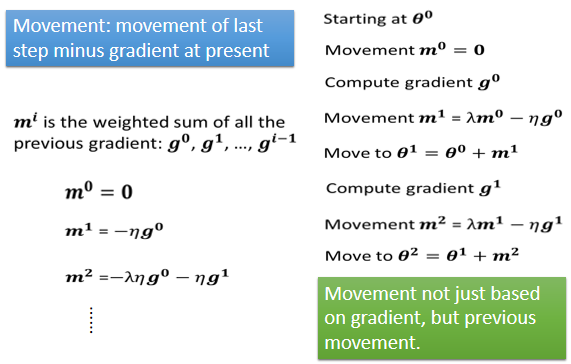
We use m to represent each step of movement, and this m can actually be written as the Weighted Sum of Gradient, which was calculated before. From the formula on the right, it can be easily seen. In fact, all m can be regarded as $\lambda \and$ related to g and then

We set m0 to 0, m1 is m0 minus g0, m0 is 0, so m1 is g0 multiplied by negative η, m2 is λ multiplied by m1, λ is another parameter, just like η is Learning Rate, we want Adjustment, λ is another parameter, this also needs to be adjusted, m2 is equal to λ multiplied by m1, minus η multiplied by g1, then where is m1, m1 is here, you can substitute m1 in, you will know m2, It is equal to negative λ multiplied by η multiplied by g0, minus η multiplied by g1, which is the Weighted Sum of g0 and g1

By analogy, so you will find that now, after adding Momentum, one interpretation is that Momentum is the negative and negative direction of Gradient plus the direction of the previous movement, but another way of interpretation is, the so-called Momentum, when adding When going to Momentum, the direction of our Update is not only to consider the current Gradient, but to consider the sum of all past Gradients.

Then we start to update the parameters from this place. According to the direction of the Gradient, we should update the parameters to the right. Now there is no direction for the previous Update, so we will completely follow the instructions given by the Gradient and move the parameters to the right. Okay, then we parameter, move a little to the right to this place

Gradient becomes very small, telling us to move to the right, but only a little bit to the right, but the previous step is to move to the right, we use a dotted line to indicate the direction of the previous step, and put it in this place, we tell the previous Gradient The direction we want to go is added to the direction of the previous step to get the direction to go to the right, then go to the right and walk to a Local Minima. It stands to reason that when you walk to a Local Minima, you can’t go forward with a Gradient or Descent. Because there is no direction of the Gradient, it is the same when walking to Saddle Point. Without the direction of the Gradient, it is impossible to move forward

But it doesn’t matter, if you have Momentum, you still have a way to continue walking, because Momentum doesn’t only look at
Gradient, Gradient is 0, you still have the direction of the previous step, the direction of the previous step tells us to go to the right, and we will continue Go right, even when you come to such a place, Gradient tells you that you should go left, but assuming that the influence of your previous step is greater than Gradient, you may still continue to go right, or even turn over a Xiaoqiu, maybe you can go to a better Local Minima, this is the possible benefit of Momentum.

According to the article

(56 messages) One of the learning skills in NN (one) parameter optimization Momentum_doubleslow;'s blog-CSDN blog_momentum parameters

As mentioned in , the speed of convergence will start to expand in other chapters.

Machine learning loss function is too large to deal with Momentum and GD

Batch and Momentum

Momentum method

Vanilla Gradient Descent general gradient descent

Gradient Descent + Momenturn

Guess you like