Matching strategy:
We have assigned many prior bboxes. If we want to predict the category and target box information, we must first know which target each prior bbox corresponds to, so that we can judge whether the prediction is accurate, and then continue the training.
The matching strategies of ground truth boxes and prior bboxes in different methods are roughly similar, but the details will be different. Here we use the matching strategy in SSD, as follows:
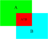
The first principle: Starting from the ground truth box, look for the priority bbox with the largest jaccard overlap with each ground truth box, so as to ensure that each ground truth box must correspond to a prior bbox (jaccard overlap is the IOU, as shown in the figure) 3, introduced earlier). Conversely, if a prior bbox does not match any ground truth, then the prior bbox can only match the background, which is a negative sample.
There are very few ground truths in a picture, but many prior bboxes. If only the first principle is matched, many prior bboxes will be negative samples, and the positive and negative samples are extremely imbalanced, so the second principle is needed.
The second principle: starting from the prior bbox, try to pair the remaining prior bbox that has not yet been paired with any ground truth box. As long as the jaccard overlap between the two is greater than the threshold (usually 0.5), then the prior bbox is also This ground truth is matched. This means that a certain ground truth may match multiple Prior boxes, which is possible. But the reverse is not possible, because a prior bbox can only match one ground truth. If multiple ground truths and the IOU of a prior bbox are greater than the threshold, then the prior bbox only matches the ground truth with the largest IOU.
Note: The second principle must be carried out after the first principle. Consider this situation carefully. If the priority bbox of the largest IOU corresponding to a certain ground truth is less than the threshold, and the matched priority bbox is the same as that of another ground truth If IOU is greater than the threshold, then who should the prior bbox match? The answer should be the former. First, make sure that each ground truth must have a prior bbox that matches it.
Use an example to illustrate the above matching principle:

There are 7 red boxes in the image representing a priori boxes, and the yellow ones are ground truths. There are three real targets in this image. Following the steps listed earlier will generate the following matches:

3.5.2 Loss function
Here is how to design the loss function.
The overall objective loss function is defined as the weighted sum of location loss (loc) and confidence loss (conf):
L(x,c,l,g) = \frac{1}{N}(L_{conf}(x,c)+\alpha L_{loc} (x,l,g)) (1)L(x,c,l,g)=N1(Lconf(x,c)+αLloc(x,l,g))(1)
Where N is the number of prior bboxes matching GT (Ground Truth), if N=0, the loss is set to 0; and the α parameter is used to adjust the ratio between confidence loss and location loss, and the default α=1 .
Confidence loss is softmax loss on multi-category confidence (c)
Where i refers to the search box serial number, j refers to the real box serial number, p refers to the category serial number, and p=0 means background. Where x^{p}_{ij}=\left\{1,0\right\}xijp={1,0} takes 1 to indicate that the i-th prior bbox matches the j-th GT box, and this GT The category of the box is p. C^{p}_{i}Cip represents the predicted probability of the category p corresponding to the i-th search box. One thing to pay attention to here, the first half of the formula is the loss of positive samples (Pos), that is, the loss of a certain category (excluding background), and the second half is the loss of negative samples (Neg), that is, the category is background. loss.
And location loss (location regression) is a typical smooth L1 loss
Among them, l is the prediction frame and g is the ground truth. (cx, xy) is the center of the default frame d after compensation (regress to offsets), and (w, h) is the width and height of the default frame. For a more detailed explanation, see the picture below:

Hard negative mining:
It is worth noting that under normal circumstances, the number of negative prior bboxes >> the number of positive prior bboxes, direct training will cause the network to pay too much attention to negative samples, and the prediction effect is very poor. In order to ensure that the positive and negative samples are as balanced as possible, we use the hard negative mining strategy used by SSD here, that is, sort the prior bboxes belonging to the negative samples according to the confidience loss, and only select the bbox with high confidience loss for training. Control the ratio of positive and negative samples to positive: negative=1:3. Its core function is to select only the difficult negative samples that are easy to be classified into the wrong category among the negative samples for network training to ensure the balance of positive and negative samples and the effectiveness of training.
For example: Suppose that among the 441 prior bboxes, P a priori boxes of positive samples and 441−P priori boxes of negative samples are obtained after matching. Arrange the negative sample prior bboxes in order of prediction loss from largest to smallest, and select the highest M prior bboxes. This M needs to be determined according to the ratio of positive and negative samples we set, for example, when we agree that the ratio of positive and negative samples is 1:3. We will take M=3P. The M negative sample hard cases with the largest loss will be used as the priority bboxes that actually participate in the calculation of loss, and the remaining negative samples will not participate in the loss calculation of the classification loss.
summary
The content introduced in this section revolves around how to conduct training, mainly three pieces:
- Matching strategy of a priori box and GT box
- Loss function calculation
- Difficult case mining
These 3 parts need to be combined to understand, we will sort out the steps to calculate loss
1) Matching a priori box and GT box
According to the scheme we introduced, each a priori box is assigned a good category to determine whether it is a positive sample or a negative sample.
Calculate loss
Calculate the classification loss and target box regression loss according to the loss function we defined
Negative samples do not calculate the regression loss of the target frame
Difficult case mining
The part of the classification loss in the loss calculated above is not the final loss
Because there are too many negative sample a priori boxes, we have to take out the part of the negative sample a priori box with the highest loss according to a certain preset ratio, generally 1:3, ignore the remaining negative samples, and recalculate the classification loss
The code of the complete loss calculation process is model.pyshown in the MultiBoxLoss category.
class MultiBoxLoss(nn.Module):
    """
    The loss function for object detection.
    对于Loss的计算,完全遵循SSD的定义,即 MultiBox Loss

    This is a combination of:
    (1) a localization loss for the predicted locations of the boxes.
    (2) a confidence loss for the predicted class scores.
    """

    def __init__(self, priors_cxcy, threshold=0.5, neg_pos_ratio=3, alpha=1.):
        super(MultiBoxLoss, self).__init__()
        self.priors_cxcy = priors_cxcy
        self.priors_xy = cxcy_to_xy(priors_cxcy)
        self.threshold = threshold
        self.neg_pos_ratio = neg_pos_ratio
        self.alpha = alpha

        self.smooth_l1 = nn.L1Loss()
        self.cross_entropy = nn.CrossEntropyLoss(reduce=False)

    def forward(self, predicted_locs, predicted_scores, boxes, labels):
        """
        Forward propagation.

        :param predicted_locs: predicted locations/boxes w.r.t the 441 prior boxes, a tensor of dimensions (N, 441, 4)
        :param predicted_scores: class scores for each of the encoded locations/boxes, a tensor of dimensions (N, 441, n_classes)
        :param boxes: true  object bounding boxes in boundary coordinates, a list of N tensors
        :param labels: true object labels, a list of N tensors
        :return: multibox loss, a scalar
        """
        batch_size = predicted_locs.size(0)
        n_priors = self.priors_cxcy.size(0)
        n_classes = predicted_scores.size(2)

        assert n_priors == predicted_locs.size(1) == predicted_scores.size(1)

        true_locs = torch.zeros((batch_size, n_priors, 4), dtype=torch.float).to(device)  # (N, 441, 4)
        true_classes = torch.zeros((batch_size, n_priors), dtype=torch.long).to(device)  # (N, 441)

        # For each image
        for i in range(batch_size):
            n_objects = boxes[i].size(0)

            overlap = find_jaccard_overlap(boxes[i], self.priors_xy)  # (n_objects, 441)

            # For each prior, find the object that has the maximum overlap
            overlap_for_each_prior, object_for_each_prior = overlap.max(dim=0)  # (441)

            # We don't want a situation where an object is not represented in our positive (non-background) priors -
            # 1. An object might not be the best object for all priors, and is therefore not in object_for_each_prior.
            # 2. All priors with the object may be assigned as background based on the threshold (0.5).

            # To remedy this -
            # First, find the prior that has the maximum overlap for each object.
            _, prior_for_each_object = overlap.max(dim=1)  # (N_o)

            # Then, assign each object to the corresponding maximum-overlap-prior. (This fixes 1.)
            object_for_each_prior[prior_for_each_object] = torch.LongTensor(range(n_objects)).to(device)

            # To ensure these priors qualify, artificially give them an overlap of greater than 0.5. (This fixes 2.)
            overlap_for_each_prior[prior_for_each_object] = 1.

            # Labels for each prior
            label_for_each_prior = labels[i][object_for_each_prior]  # (441)
            # Set priors whose overlaps with objects are less than the threshold to be background (no object)
            label_for_each_prior[overlap_for_each_prior < self.threshold] = 0  # (441)

            # Store
            true_classes[i] = label_for_each_prior

            # Encode center-size object coordinates into the form we regressed predicted boxes to
            true_locs[i] = cxcy_to_gcxgcy(xy_to_cxcy(boxes[i][object_for_each_prior]), self.priors_cxcy)  # (441, 4)

        # Identify priors that are positive (object/non-background)
        positive_priors = true_classes != 0  # (N, 441)

        # LOCALIZATION LOSS

        # Localization loss is computed only over positive (non-background) priors
        loc_loss = self.smooth_l1(predicted_locs[positive_priors], true_locs[positive_priors])  # (), scalar

        # Note: indexing with a torch.uint8 (byte) tensor flattens the tensor when indexing is across multiple dimensions (N & 441)
        # So, if predicted_locs has the shape (N, 441, 4), predicted_locs[positive_priors] will have (total positives, 4)

        # CONFIDENCE LOSS

        # Confidence loss is computed over positive priors and the most difficult (hardest) negative priors in each image
        # That is, FOR EACH IMAGE,
        # we will take the hardest (neg_pos_ratio * n_positives) negative priors, i.e where there is maximum loss
        # This is called Hard Negative Mining - it concentrates on hardest negatives in each image, and also minimizes pos/neg imbalance

        # Number of positive and hard-negative priors per image
        n_positives = positive_priors.sum(dim=1)  # (N)
        n_hard_negatives = self.neg_pos_ratio * n_positives  # (N)

        # First, find the loss for all priors
        conf_loss_all = self.cross_entropy(predicted_scores.view(-1, n_classes), true_classes.view(-1))  # (N * 441)
        conf_loss_all = conf_loss_all.view(batch_size, n_priors)  # (N, 441)

        # We already know which priors are positive
        conf_loss_pos = conf_loss_all[positive_priors]  # (sum(n_positives))

        # Next, find which priors are hard-negative
        # To do this, sort ONLY negative priors in each image in order of decreasing loss and take top n_hard_negatives
        conf_loss_neg = conf_loss_all.clone()  # (N, 441)
        conf_loss_neg[positive_priors] = 0.  # (N, 441), positive priors are ignored (never in top n_hard_negatives)
        conf_loss_neg, _ = conf_loss_neg.sort(dim=1, descending=True)  # (N, 441), sorted by decreasing hardness
        hardness_ranks = torch.LongTensor(range(n_priors)).unsqueeze(0).expand_as(conf_loss_neg).to(device)  # (N, 441)
        hard_negatives = hardness_ranks < n_hard_negatives.unsqueeze(1)  # (N, 441)
        conf_loss_hard_neg = conf_loss_neg[hard_negatives]  # (sum(n_hard_negatives))

        # As in the paper, averaged over positive priors only, although computed over both positive and hard-negative priors
        conf_loss = (conf_loss_hard_neg.sum() + conf_loss_pos.sum()) / n_positives.sum().float()  # (), scalar

        # return TOTAL LOSS
        return conf_loss + self.alpha * loc_loss
Original link: https://datawhalechina.github.io/dive-into-cv-pytorch/#/chapter03_object_detection_introduction/3_5