Spiking Neural Network - Handwritten Digit Recognition Based on IAF Neurons

1. Implementation method of spiking neural network

With the popularity of Neuromorphic Technology, more and more engineers and academic researchers are investing in the field of pulsed nerves. Congratulations~~

In order to facilitate the research and development and engineering of spiking neural networks, more and more excellent implementation frameworks of spiking neural networks have been gradually developed, but because the industry itself is still in the process of development, in fact, there is no such thing as pytorch/tensorflow in the industry It is also regarded as the industry standard SNN development framework.

As mentioned in the previous blog post, the current spiking neural network still needs a stable learning algorithm that can fully reflect its advantages. Based on the ease of learning and ease of use, this blog post mainly describes a method of implementing a spiking neural network using the ANN-SNN conversion method. This method is very suitable for children's shoes with a deep learning background. It mainly has the following Several advantages:

• Based on the mature Pytroch framework, it is easy to use and the installation package is simple, allowing everyone to focus on researching SNN
• Based on BP, the learning method is mature and stable, and there are a lot of open source materials. After all, gradient descent supports the entire neural network.
• The performance is stable, the basic ANN can become our SNN, and it will not fail to work due to inexplicable algorithms

Of course, there are also disadvantages:

• Generally dissed: not close to biological characteristics at all (it’s easy to use Hhhhh)
• Based on rate coding, the number of pulses generated by the middle layer of the neural network is too large, which generally does not have the characteristics of low power consumption
• The conversion process will cause accuracy loss due to approximate estimation, but it is generally stronger than networks trained with algorithms such as STDP

2. Sinabs

Here is an introduction to Sinabs , a spiking neural network framework with Pytorch as the backend, short and concise, concise but not simple~

Installation: In the python3 environment:

pip install sinabs

3. IAF (Integrate and Fire) neurons

Compared with LIF neurons, IAF neurons have one less leakage item of membrane voltage, the expression is as follows:
$$t\dot{v}=R\cdot (I_{syn}+{\tilde{I}}_{bias})$$

When the neuron modulus voltage threshold is set to 1, for a synaptic input with a constant input size, the membrane voltage change can be displayed as the following figure:

IAF is a relatively simple model in the current spiking neurons. It does not have the operation term of leaking modulus voltage over time, so the membrane voltage in IAF neurons will only have two changes: linear rise and instantaneous reset. But it also has the property of converting the corresponding input into a modulo voltage change and comparing it with a threshold. Each spike neuron has its corresponding membrane voltage (or state-state) over time t, which is the biggest difference between spike neurons and traditional artificial neurons.

4. Principle of ANN-SNN

Bodo et al. proposed a complete and feasible ANN-SNN conversion framework in
Conversion of Continuous-Valued Deep Networks to Efficient Event-Driven Networks for Image Classification
. The theory that Sinabs relies on is also changed from this article. Here is a rough explanation:

The number of output pulses of LIF and IAF spiking neurons within a limited time window or their firing rate is linearly proportional to the synaptic input current they receive. If you simply draw the relationship between firing rate VS synaptic output, it should be as shown in the figure below:

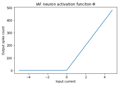
That's right, students who are familiar with deep neural networks have discovered, isn't this the same as ReLU? The feasibility of ANN-SNN conversion is reflected here. After training ANN, we only need to map the commonly used ReLU activation equation in ANN to the pulse frequency of SNN.

On top of this, Bodo and other great gods proposed a series of methods that can convert commonly used ANN operations such as BN, pooling, into event-driven methods to improve the trainability of SNN. At the same time, during the conversion process, there are many small tricks that can improve the efficiency and stability of the conversion network. I won’t go into details here. Interested students can read the details in the article.

5. Handwritten digit recognition based on Sinabs framework

With the above principles, we can practice a handwritten digit recognition task. However, this time, the difference from the traditional grayscale image is that we will directly use the data provided by the event camera. After all, because of the natural fit between the spiking neural network and the event camera, processing event data is what the spiking neural network should do.

We are using the Neuromorphic MNIST database this time, and its source is:

https://www.garrickorchard.com/datasets/n-mnist

The data is completely derived from the real dynamic visual event camera, and the corresponding data processing has been done. It is characterized by sparse asynchronous, discrete in the time domain, and has extremely high time resolution (events and event intervals can reach the lowest ns level) .

Note: For the preprocessing of AER data, this article will not show too much, let us focus on the implementation of SNN itself for the time being. If there is a need, I will write a blog post on how to process event data later.

First of all, we need to make it clear that in the simulation process of SNN, the representation of time is still discrete, and we need to establish a simulation network based on time-step. Ideally, the operation of the spiking neural network should be completely asynchronous, without sampling frequency.

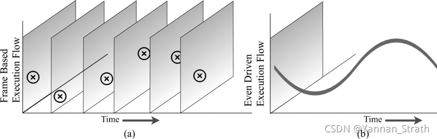
To give a more specific example, traditional sensors such as RGB cameras generally have a fixed sampling frequency, such as 30FPS. So for the neural network, its calculations are also performed on a frame-by-frame picture. The operation of each spike neuron of the event-driven SNN should be independent of each other (in time and space).

[1] 图： Frame based vs Event-driven processing

Based on these two points:

• Simulate operations in frames
• The number of pulses corresponds to the corresponding ReLU activation function.
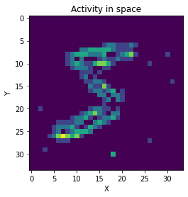
  Our input data will be a compressed matrix of one frame within a limited time window. For N-MNIST data, it is 2x34x34, and the corresponding true value on each pixel It is the number of pulses generated by the corresponding position within the time window, and channel 2 is the on/off polarity.
  If visualized it looks like this:
  

So let's build a simple CNN first, using pytorch's SequentialAPI is very simple:

import torch.nn as nn

cnn = nn.Sequential(
    nn.Conv2d(2, 20, 5, 1, bias=False),
    nn.ReLU(),
    nn.AvgPool2d(2,2),
    nn.Conv2d(20, 32, 5, 1, bias=False),
    nn.ReLU(),
    nn.AvgPool2d(2,2),
    nn.Conv2d(32, 128, 3, 1, bias=False),
    nn.ReLU(),
    nn.AvgPool2d(2,2),
    nn.Flatten(),
    nn.Linear(128, 500, bias=False),
    nn.ReLU(),
    nn.Linear(500, 10, bias=False),
    nn.ReLU()
)

So far, we can also train this network completely according to the method of ANN

device = "cuda" if torch.cuda.is_available() else "cpu"
cnn = cnn.to(device) # GPU
optimizer = torch.optim.Adam(ann.parameters(), lr=1e-3)
n_epochs = 1
for n in range(n_epochs):
    # Iterate over data
    for data, target in train_data:
        data, target = data.to(device), target.to(device) # GPU
        output = cnn(data) # forward pass through the network
        optim.zero_grad()

        # Add loss to the total loss
        loss = F.cross_entropy(output, target)

        # Propagate loss backwards
        loss.backward()

        # Update weights
        optimizer.step()

        # get the index of the max log-probability
        pred = output.argmax(dim=1, keepdim=True)

        # Compute the total correct predictions
        correct = pred.eq(target.view_as(pred)).sum().item()
# Save model parameters
torch.save(ann.state_dict(), "ann.pt")

After ANN training and fitting, we can use the api of sinabs to convert ann to snn in just one sentence

from sinabs.from_torch import from_model
input_shape = (2, 34, 34)
sinabs_model = from_model(snn, input_shape=input_shape, add_spiking_output=True)

So what did he do? In fact, sinabs_modelit is still a pytorch model, which contains analog_modeland spiking_modelcorresponds to the original ann model and the converted snn model respectively. The weights of the trained convolutional layer and the fully connected layer are exactly the same, the only difference is the way of activation, where spiking_modelReLU is replaced by a corresponding layer SpikingLayer(). This layer of neurons defaults to the IAF neuron type. When testing, if you call it, sinabs_model.spiking_model(input)the model will use snn for testing by default. The value generated by the convolution operation can be understood as the synaptic current generated by the input pulse after the pulse convolution operation, and then converted into the corresponding membrane voltage change after passing through the membrane resistance R=1.

sinabs_model.spiking_model

Sequential(
  (0): Conv2d(2, 20, kernel_size=(5, 5), stride=(1, 1), bias=False)
  (1): SpikingLayer()
  (2): AvgPool2d(kernel_size=2, stride=2, padding=0)
  (3): Conv2d(20, 32, kernel_size=(5, 5), stride=(1, 1), bias=False)
  (4): SpikingLayer()
  (5): AvgPool2d(kernel_size=2, stride=2, padding=0)
  (6): Conv2d(32, 128, kernel_size=(3, 3), stride=(1, 1), bias=False)
  (7): SpikingLayer()
  (8): AvgPool2d(kernel_size=2, stride=2, padding=0)
  (9): Flatten(start_dim=1, end_dim=-1)
  (10): Linear(in_features=128, out_features=500, bias=False)
  (11): SpikingLayer()
  (12): Linear(in_features=500, out_features=10, bias=False)
  (13): SpikingLayer()
)

At this time, when we conduct SNN tests, it becomes very unrealistic to use a single frame. Because a real snn should accept an asynchronous input signal, not the number of pulses accumulated over a period of time. At this time, our usual practice is to set the time step to be very small so that the original frame becomes a (T/time_step) frame. For example, when we trained ANN, we used an equivalent compressed frame of 50ms per frame. During the test Correspondingly, if the time_step we choose is 1ms, then the dimension of the test sample should be (50, 2, 34, 34), and if it is 100us, it corresponds to (500, 2, 34, 34). Theoretically speaking, the smaller the time_step is, the closer it is to the actual pulse sequence. The optimal value should be within each time_step, the value of any pixel $\in [0,1]$ . Of course, this will also cause the calculation time to be too long.

On top of this, we test the network:

Select a sample of the test set:

raster, label = dataset_test_spiketrains[54]
print(label)
print(raster.shape)

4
(300, 2, 34, 34)

Here we choose 1ms as the time_step, you can see that the shape of a sample is (300, 2, 34, 34). When outputting, we will also weight the t dimension, because this is a sample continuous output result.

test

for data, target in tqdm(dataloader_test_spiketrains):
    sinabs_model.reset_states()
    
    data = data[0].to(device)
    output = sinabs_model(data)
    
    # we sum the number of output spikes in time for each sample
    output = output.sum(axis=0) # (135, 10)

    # get the index of the max log-probability
    pred = output.argmax() # which neuron spikes most

    # Compute the total correct predictions
    correct = pred.item() == target.item()
    
    acc.append(correct)
    
    # let's stop at 200 samples, otherwise it takes too long
    if len(acc) > 200:
        break

Let's take a look at what the network has done:

raster, label = dataset_test_spiketrains[54]

# plot it in space: this is the same as the frame,
# we remove the time dimension
plt.title("Input spikes in space")
plt.imshow(raster.sum((0, 1)))
plt.xlabel("X")
plt.ylabel("Y");

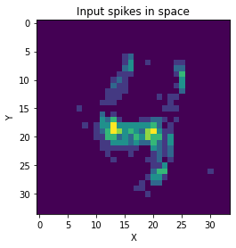
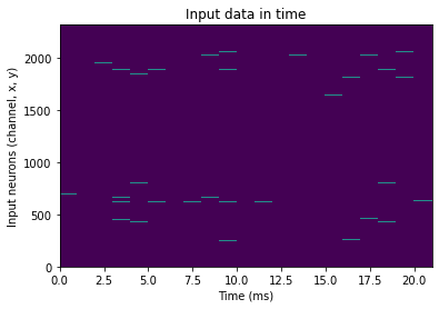
Here we look at the input:

plt.title("Input data in time")
plt.pcolormesh(raster.reshape((-1, 2*34*34)).T)
plt.xlabel("Time (ms)")
plt.ylabel("Input neurons (channel, x, y)");

For output:

output.T.detach().numpy()

The 2-dimensional matrix we got (300, 10) where 300 corresponds to time and 10 corresponds to the label of MNIST

Because this SNN is rate-based, then in 300 time steps, we find the spike neuron corresponding to the most spikes, which is the output prediction of the network for this input.

If everything is OK, then we will find that the test accuracy of SNN will be much lower than that of ANN!

This is because the SNN itself will have a situation where the activation value does not correspond to the number of pulses after conversion. The output of the pulse neuron is shaped. For example, ReLU can generate an activation value like 2.13324, and the pulse can only be 1. 2, 3...

In this case, we generally increase the activity of the entire spike network, because of the linear relationship in the positive area, we can directly increase the weight in proportion to make the activation function of the ann and the snn match each other as much as possible.

Due to space reasons, we use Sinabs to implement ANN-SNN method here first, hope it can help everyone.

Finally, it is strongly recommended to read the sinabs documentation:
https://sinabs.ai

Bodo神的paper:
Rueckauer, B., Lungu, I. A., Hu, Y., Pfeiffer, M., & Liu, S. C. (2017). Conversion of continuous-valued deep networks to efficient event-driven networks for image classification. Frontiers in neuroscience, 11, 682.

[1]https://www.researchgate.net/figure/Comparison-of-frame-based-and-event-based-processing-The-circles-on-the-Frame-based_fig3_342133982