Super-resolution algorithm ESRT: Transformer for Single Image Super-Resolution

The network structure ESRT (Efficient Super-Resolution Transformer) in this article is quite complicated, and it is a combination of CNN and Transformer. The article proposes an efficient SRTransformer structure, which is aLightweight Transformer. The author considers that similar details in an image in image super-resolution can be used as a reference supplement (similar to super-resolution based on the reference image Ref), so the Transformer is introduced to model a long-term dependency in the image. However, these ViT methods are too computationally intensive and take up too much memory, so this lightweight version of the Transformer structure (ET) was proposed, ET只使用了transformer中的encoderand the author also used feature spiltthe QKV to be divided into groups to calculate the attention and finally splicing. The article also proposes one in the CNN part 高频滤波器模块HFM, which retains high-frequency information for feature extraction.

The main focus of the article is speed (high efficiency), and the effect is also very good. In the experimental part, the author mentioned that grafting the ET structure into RCAN can also improve the effect of RCAN, which proves the effectiveness of ET.

Original link: ESRT: Transformer for Single Image Super-Resolution
Source code address: https://github.com/luissen/ESRT.

Abstract

With the development of deep learning, single image super-resolution (SISR) technology has made great progress. Recently, more and more researchers have begun to explore the application of Transformer in computer vision tasks. However, Vision Transformer's huge computational cost and high GPU memory footprint hinder its progress. In this paper, a novel efficient super-resolution Transformer (ESRT) for SISR is proposed. ESRT is a hybrid model consisting of 轻型CNN主干网（LCB）and 轻型Transformer主干网（LTB）. Among them, LCB can dynamically adjust the size of feature maps to extract deep features with lower computational cost. LTB consists of a series of efficient Transformers (ETs), using a specially designed efficient multi-head attention (EMHA), which occupies very little GPU memory. Extensive experiments show that ESRT achieves competitive results at a lower computational cost. Compared with the original Transformer occupying 16057M GPU memory, ESRT only occupies 4191M GPU memory.

1 Introduction

Because similar image patches in the same image can be used as reference images for each other , so that the texture details of a specific patch can be recovered using the reference patch. Inspired by this, the author introduces Transformer into the SISR task, because Transformer has a strong feature expression ability and can model such long-term dependencies in images . The goal is to explore the feasibility of using Transformer in lightweight SISR tasks. Recently several Transformers have been proposed for computer vision tasks. However, these methods often occupy a large amount of GPU memory , which greatly limits their flexibility and application scenarios.

To address the above issues, an Efficient Super-Resolution Transformer (ESRT) is proposed to enhance the ability of SISR networks to capture long-distance context dependencies while significantly reducing the memory cost of GPUs .

ESRT is a hybrid architecture that uses the "CNN+Transformer" model to process small SR datasets. ESRT can be divided into two parts: Lightweight CNN Backbone (LCB) and Lightweight Transformer Backbone (LTB).

1. For LCB, more consideration is given to reducing the shape of feature maps in the middle layers and maintaining a deep network depth to ensure a large network capacity. Inspired by high-pass filters, one is designed 高频滤波模块（HFM）to capture the texture details of images . In HFM, another method is proposed 高保留块（HPB）to effectively extract latent features through size changes. In terms of feature extraction, a powerful basic feature extraction unit is proposed 自适应残差特征块（ARFB）, which can adaptively adjust the residual path and the weight of the path.
2. In LTB, one is proposed 高效Transformer(ET), which uses a specially designed Efficient Multi-Head Attention (EMHA) mechanism to reduce GPU memory consumption. And only consider the relationship between image patches in local regions , because pixels in SR images are usually related to their neighbors. Although it is a local region, it is much wider than regular convolutions and can extract more useful contextual information. Therefore, ESRT can effectively learn the relationship between similar local patches, enabling super-resolved regions to have more references.

The main contributions are as follows:

1. A lightweight CNN backbone (LCB) is proposed that uses high-preservation blocks (HPB) to dynamically resize feature maps to extract deep features with low computational cost
2. A Lightweight Transformer Backbone (LTB) is proposed to capture long-term dependencies between similar patches in an image using a specially designed Efficient Transformer (ET) and Efficient Multi-Head Attention (EMHA) mechanism
3. A new model called Efficient SR Transformer (ESRT) is proposed to effectively enhance the feature expressiveness and long-term dependencies of similar patches in images, achieving better performance with lower computational cost.

2 Efficient Super-Resolution Transformer

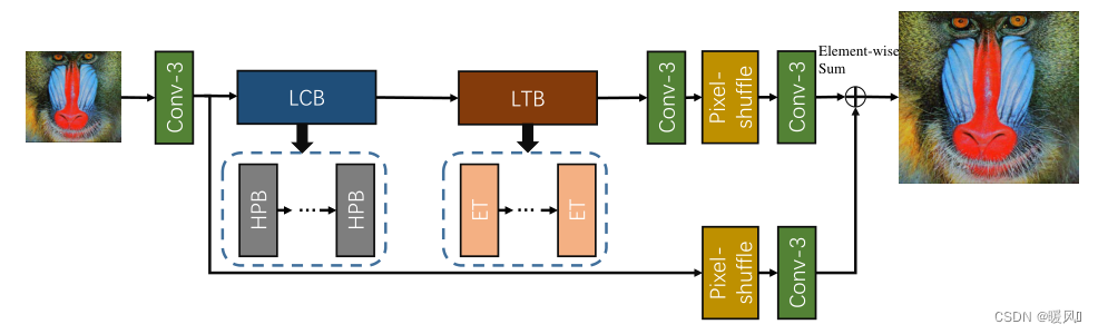
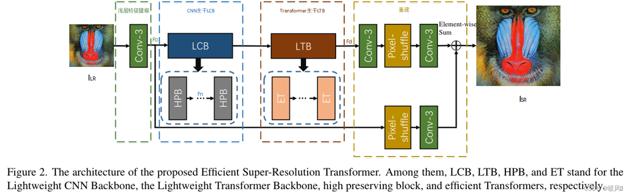
Efficient Super-Resolution Transformer (ESRT) mainly consists of four parts: shallow feature extraction, lightweight CNN backbone (LCB), lightweight Transformer backbone (LTB) and image reconstruction.

Shallow feature extraction:
a 3×3 convolutional layer

Lightweight CNN Backbone (LCB):
Consists of multiple High Preserving Blocks (HPBs) (3 in the experiment), $g^n$ is the mapping of the nth HPB,the output of the nth HPB is$F_n$,official:

Lightweight Transformer Backbone (LTB):
The output of each HPB is concatenated and sent to the LTB fusion feature. The LTB consists of multiple Efficient Transformers (ETs) (1 in the experiment), $\varphi$ represents the function of ET,$F_d$is the output of LTB, the formula is as follows .

Image reconstruction:
final $F_d$and $F_0$At the same time, it is fed into the reconstruction module to obtain the reconstructed image $I_{SR}$。$f$ and$f_p$Represent the convolutional layer and the sub-pixel convolutional layer respectively, and obtain $I_{SR}$The formula is as follows:

The overall structure of ESRT is relatively conventional, and deep feature extraction uses CNN and Transformer jointly. A relatively complex structure is used in LCB, and the reasoning speed is relatively slow, while only one Transformer encoder structure is used in ET, which does not bring too much calculation. Later experiments also proved that adding ET can bring benefits to the network.

2.1 Lightweight CNN Backbone (LCB)

The role of the Lightweight CNN Backbone (LCB) is to extract latent image features in advance, enabling the model to have the initial capability of super-resolution . LCB mainly 高保留块（HPB）consists of a series.

HPB:
Previous SR networks usually keep the spatial resolution of the feature map unchanged during processing. In this paper, to reduce the computational cost , a novel High Preservation Block (HPB) is proposed to reduce the resolution of processed features . However, the reduction in feature map size often results in the loss of image details, resulting in visually unnatural reconstructed images. In order to solve this problem, in HPB, the author creatively proposes 高频滤波模块（HFM）and 自适应残差特征块（ARFB）.

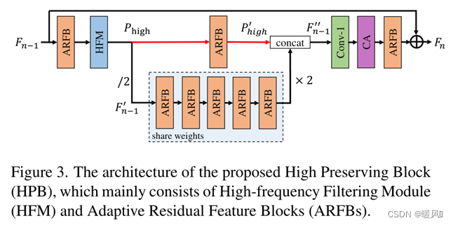
First introduce the overall structure of HPB: it consists of HFM and ARFB. Then analyze the structure of HFM and ARFB in detail.

the whole frame: Output F n − 1 F_{n-1} of the previous HPB$F_{n-1}$, as the input of the current HPB. First go through a ARFBmethod for extracting $F_{n-1}$as an input function to the HFM. Then, use HFMthe high-frequency information of the calculated features (marked as $P_{high}$). After getting $P_{high}$Finally, the size of the feature map is reduced to reduce computational cost and feature redundancy. 下采样The feature map is expressed as $f_{n-1}^{\prime }$, for $f_{n-1}^{\prime }$Use 多个共享权重的ARFBto explore the latent information of SR images (reduce parameters). At the same time, use 单个ARFBthe processing $P_{high}$To align the feature space $f_{n-1}^{\prime }$。$f_{n-1}^{\prime }$After feature extraction 上采样to the original size via bilinear interpolation. 拼接融合$f_{n-1}^{\prime }$和$P_{high}^{\prime }$, get $f_{n-1}^{\prime \prime }$, to preserve the initial details. Get $f_{n-1}^{\prime \prime }$The formula of is:

Among them, ↑ and ↓ represent up and down sampling; $f_a$Represents the function of ARFB. To balance model size and performance, five ARFBs with shared parameters are employed.

$f_{n-1}^{\prime \prime }$Concatenated by two features, so use it first 1×1卷积层to reduce the number of t channels. Then, use 通道注意力to weight channels with high activation values. Finally, the final features are extracted using ARFB and proposed 全局残差连接to add the original features $F_{n-1}$to $F_n$. The purpose of this operation is to learn residual information from the input and stabilize training.

The channel attention module is quoted from the article Squeeze-and-excitation networks, or it is the same as the CA module used in RCAN .

This article is actually a Matryoshka residual structure, but many improvements have been made in the residual structure, such as adding adaptive Res scaling, high-frequency filters, down-sampling circular convolution, and so on.

HFM：High-frequency Filtering Module

Since Fourier transform is difficult to embed in CNN, this paper proposes one 可微HFM. The goal of HFM is to estimate the high-frequency information of the image from the LR space .

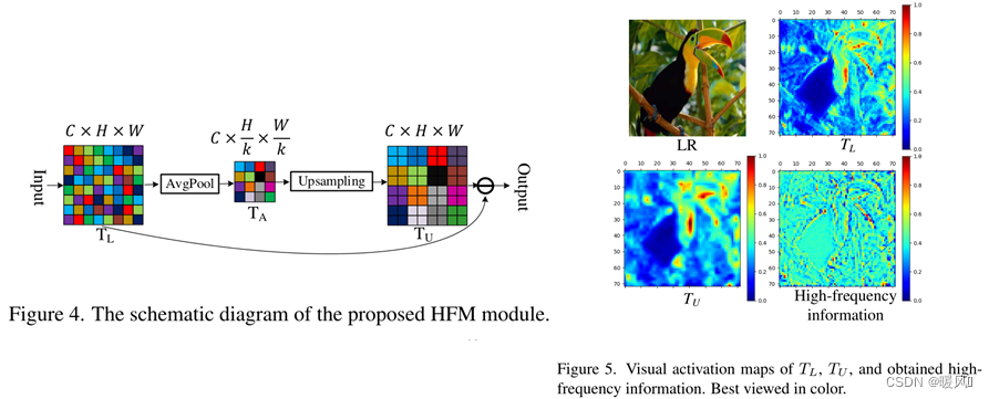
As shown in Figure 4, suppose the input feature map $T_L$The size is $C\times H\times W$ , first平均池化obtain$T_A$:

where k represents the kernel size of the pooling layer, and the intermediate feature map $T_A$The size is $C\times \frac{H}{k}\times \frac{W}{k}$。$T_A$Each value in can be treated as a specified $T_L$The average intensity of a small area. Afterwards, TA is performed 上采样to obtain the dimensions $C\times H\times$new tensorTU T_U$of\; W$$T_U$。$T_U$is the expression for the average smoothness information. Finally, from $T_L$中按元素减去$T_U$to obtain high-frequency information.

$T_L$、$T_U$The visual activation map of the and high-frequency information is shown in Fig. 5. It can be observed that $T_U$than $T_L$smoother as it is $T_L$average information. Meanwhile, high-frequency information preserves the details and edges of feature maps before downsampling (average pooling). Therefore, it is crucial to preserve this information.

ARFB：Adaptive Residual Feature Block

Inspired by ResNet and VDSR, when the depth of the model increases, 残差结构it can alleviate the gradient disappearance problem and increase the representation ability of the model. So a block (ARFB) is proposed 自适应残差特征as the basic feature extraction block.

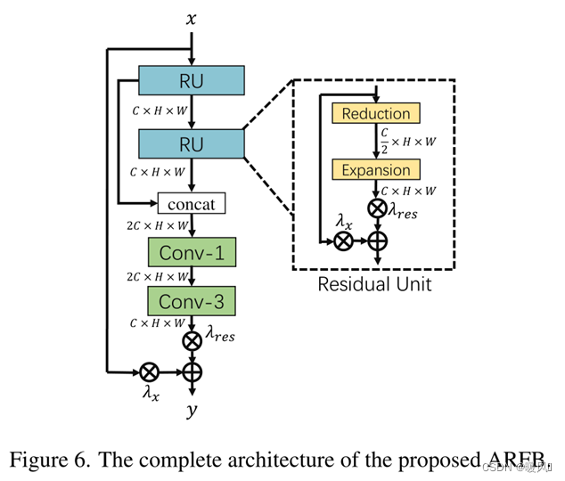
ARFB contains two residual units (RU) and two convolutional layers. To save memory and number of parameters, RU consists of two modules: a reduction module and an expansion module . For reductions, 将特征映射的通道减少一半, and restores for expansions. At the same time, a Residual Scaling Algorithm (RSA) with adaptive weights is designed to dynamically adjust the residual path weights. Compared with fixed Res scaling, RSA can improve the flow of gradients and automatically adjust the content of the residual feature map for the input feature map. Suppose $x_{ru}$is the input of RU, the process of RU can be expressed as :

Among them, $y_{ru}$is the output of RU, $f_{re}$and $f_{ex}$Represents the reduction and expansion operations, $l_{res}$和$l_x$are the adaptive weights of the two paths, respectively. Use 1×1卷积层to vary the number of channels for reduction and expansion functions. At the same time, the outputs of two RUs are concatenated and input 1×1卷积层to make full use of hierarchical features . Finally, channels are used 3×3卷积层to reduce the feature maps and extract effective information from the fused features .

LCB, the part of CNN is over, review: LCB is composed of three HPB. Each HPB is composed of HFM and ARFB, and the structure includes channel attention and ARFB with up and down adoption and five shared parameters. A concept runs through the whole text: reduce parameters. (ARFB shared parameters, up and down sampling, and reduced expansion layers are all to reduce parameters and reflect light weight and high efficiency )

 

---

2.3 Lightweight Transformer Backbone (LTB)

In SISR, similar image blocks in an image can be used as reference images for each other, so other image blocks can be referred to to restore the texture details of the current image block, which is very suitable for using Transformer . However, previous vision Transformer variants usually require a large amount of GPU memory , which hinders the development of Transformer in the vision field. In this paper, the authors propose a Lightweight Transformer Backbone (LTB). LTB consists of specially designed efficient Transformers (ETs), which can capture the long-term dependencies of similar local regions in images with low computational cost .

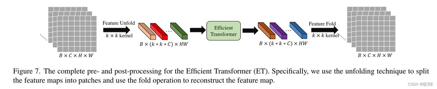
Preparatory work before and after: expand the feature map into a one-dimensional sequence, and convert the sequence back to the feature map

The standard Transformer takes a one-dimensional sequence as input and learns the long-distance dependencies of the sequence. Whereas for vision tasks, the input is always a 2D image .

In ViT, 1D sequences are generated by partitioning non-overlapping blocks , which means that there is no pixel overlap between each block. The authors believe that this preprocessing method is not suitable for SISR.

Therefore, a new feature map processing method is proposed. As shown in Figure 7, the feature map is divided into small pieces using the unfolding technique (in fact, overlapping blocks are used to divide the patch ), and each small piece is regarded as a "word". Specifically, feature map $\in R^{C\times H\times W}$ (by$k\times k$ core) is expanded into a series of patches, namely$F_{pi}\in R^{k^2\times C}，i=1，\dots ,N$ , where$N=H\times W$ is the number of patches. The key part is that the number of N is$H\times W$ , means each k × kk×kwhen splitting$k\times The\; kernel\; movement\; step\; of\; k$ is 1, and there is a large overlap between each patch. Both ViT and Swin-T are divided by non-overlapping blocks, and the number of N obtained is$\frac{H}{k}\times \frac{W}{k}$。

The author said that since the "unfold" operation will automatically reflect the position information of each patch, the learnable position embedding of each patch will be eliminated (??? This is eliminated). These patches are then sent directly to ET. The output of ET has the same shape as the input , and the "fold" operation is used to reconstruct the feature map.

 
EMHA: Efficient Multi-Head Attention

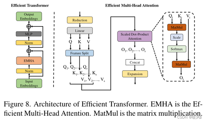
is simple and efficient . Like ViT, ET only uses the standard Transformer encoder structure. As shown on the left of Figure 8, in the encoder of ET, there is an efficient multi-head attention (EMHA) and an MLP. Meanwhile, layer normalization is used before each block, and residual connections are applied after each block. The ET part is basically the same as the standard encoder structure. The only difference is that ① the author divides the QKV features into s groups, and each group performs attention to obtain the output O i $O_i$, then Concat the output to O. Split the multiplication of large matrices into multiple multiplications of small matrices to reduce parameter operations; ② mask is not applicable to attention calculations.

As shown on the right side of Figure 8, suppose the input $E_i$has the shape B×C×N.

1. First, reduce the number of channels缩减层 by half using ( B × C 2 × NB×\frac{C}{2}×N$B\times \frac{C}{2}\times N$）。
2. Then, a feature map is projected into three elements线性层 : Q (query), K (key) and V (value) by a .
3. Use 特征分割the (FS) module to split Q, K, and V into s segments with the same split factor s , denoted as $Q_1,...,Q_s$、$K_1,...,K_s$和$V_1,...,V_s$。
4. 对应的$Q_i,K_i,V_i$Separately calculate 注意力操作(SDPA) output $O_i$, SDPA omits the mask operation compared to the standard attention module.
5. General $O_1,O_2,\dots ,O_s$拼接up, generating the entire output feature O.
6. Use 扩展层the recovery channel number at the end .

Assuming that in the standard Transformer, Q and K calculate a self-attention matrix with a shape of B×m×N×N. Then this matrix is ​​combined with V to calculate self-attention, and the 3rd and 4th dimensions are N×N. For SISR, images usually have high resolution , resulting in very large N , and the computation of the self-attention matrix consumes a lot of GPU memory and computational cost.
↓↓ To solve this problem, Q, K, and V are segmented into s equal segments
since prediction pixels in super-resolution images usually only depend on local neighbors in LR. The 3rd and 4th dimensions of the last self-matrix become $\frac{N}{s}\times \frac{N}{s}$, significantly reducing the amount of computation and GPU storage costs .

3 Experiments

setting：

Training: Use DIV2K as the training dataset.
Testing: Five benchmark datasets were used, including Set5, Set14, BSD100, Urban100, and Manga109 .
Metrics: PSNR and SSIM are used to evaluate the performance of reconstructed SR images.
batch: 16
patch: 48×48
image enhancement: random horizontal flip and 90 degree rotation
initial learning rate is set to $2\times 10^{-4}$ is halved every 200 epochs.
optimizer: Adam, momentum = 0.9.
Loss function: L1 loss
takes about two days to train with a GTX1080Ti GPU.

The reduction layer uses a 1×1 convolution kernel, and the others use a 3×3
convolution layer with 32 channels and a fusion layer with 64 channels. Image
reconstruction uses PixelShuffle
HFM with k = 2,
three HPBs, and an ET
split factor s = 4
ET k = 3
EMHA 8-head attention in before and after work

3.1 Comparisons with Advanced SISR Models

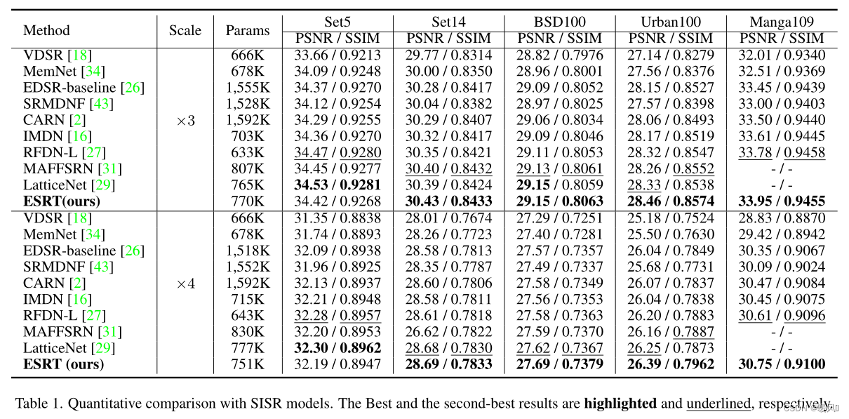
In Table 1,

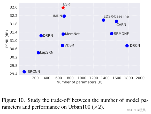
1. Although the performance of the EDSR baseline is close to that of ESRT, its parameters are almost twice that of ESRT.
2. The parameters of MAFFSRN and LatticeNet are close to ESRT, but the results of ESRT are better than them.
3. ESRT performs much better on Urban100 than other models. This is because there are many similar patches in each image of this dataset. Therefore, the LTB introduced in ESRT can be used to capture the long-term dependencies between these similar image patches and learn their correlations to achieve better results.
4. At ×4 scale, the gap between ESRT and other SR models is more obvious . This is aided by the effectiveness of the proposed ET, which can learn more from other clear domains.
5. All these experiments verify the effectiveness of the proposed ESRT .
   

3.2 Comparison on Computational Cost

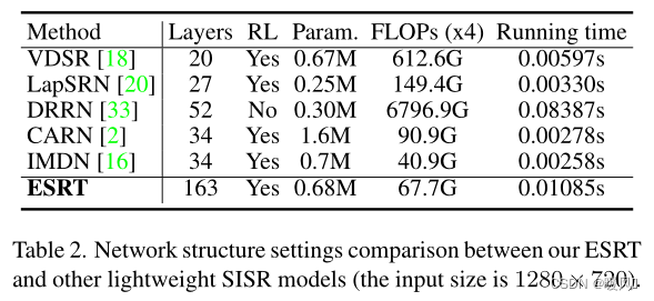
In Table 2,

1. ESRT can go up to 163 layers and still achieves the second lowest hash rate (67.7G) among these methods. This benefits from the proposed HPB and ARFB, which can effectively extract useful features and preserve high-frequency information.
2. Even though ESRT uses Transformer architecture, the running time is very short . The increased time compared to CARN and IMDN is perfectly acceptable.
   

3.3 Ablation Study

HPB:
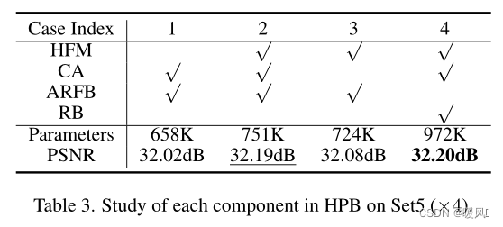
Table 3 explores the effectiveness of the HPB components of ESRT .

1. Comparing Case1, 2, and 3, it can be observed that the introduction of HFM and CA can effectively improve the performance of the model, but will increase the parameters.
2. Comparing Case2 and 4, it can be seen that if RB is used instead of ARFB, the PSNR result is only increased by 0.01dB, but the number of parameters is increased to 972K. This means that ARFB can significantly reduce model parameters while maintaining excellent performance .
3. All these results fully demonstrate the necessity and effectiveness of these modules and mechanisms in HPB.

ET:
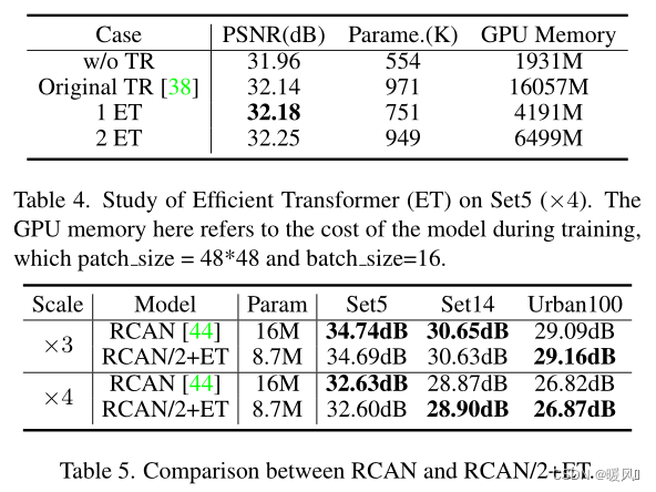
In Table 4, the influence of Transformer on the model is analyzed .

1. If ESRT removes the Transformer, the model performance will drop significantly from 32.18dB to 31.96dB. This is because the introduced Transformer can make full use of the relationship between similar image patches in the image.
2. ET is compared with the original Transformer in the table. 1ET achieves better results with fewer parameters and GPU memory consumption (1/4). Experiments fully verify the effectiveness of the proposed ET.
3. As the number of ETs increases, the model performance will further improve. However, it is worth noting that model parameters and GPU memory also increase with the number of ETs. Therefore, to achieve a good balance between model size and performance, only one ET is used in the final ESRT.

To verify the effectiveness and generalizability of the proposed ET , ET is introduced into RCAN. The authors only use a small version of RCAN (the number of residual groups is set to 5) in the experiment, and add ET before the reconstruction part. It can be seen from Table 5 that the performance of the "RCAN/2+ET" model is close to or even better than that of the original RCAN with fewer parameters. This further demonstrates the effectiveness and generality of ET, which can be easily ported to any existing SISR model to further improve the model's performance.

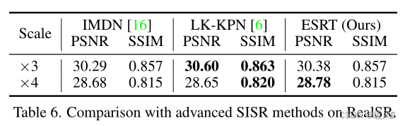
3.4 Real Image Super-Resolution

ESRT compared with some classic lightweight SR models on real image dataset ( RealSR ). According to Table 6, it can be observed that ESRT achieves better results than IMDN. Furthermore, ESRT outperforms LK-KPN on ×4, which is specially designed for practical SR tasks. This experiment further verifies the effectiveness of ESRT on real images.

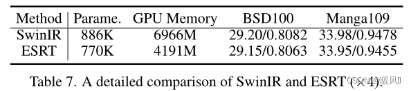
3.5 Comparison with SwinIR

EMHA in ESRT is similar to Swin-Transformer layer of SwinIR . However, SwinIR uses sliding windows to solve the high computation problem of Transformer , while ESRT uses splitting factors to reduce GPU memory consumption . According to Table 7, compared with SwinIR, ESRT achieves close performance with less parameters and GPU memory. It is worth noting that SwinIR uses an additional dataset ( Flickr2K ) for training, which is the key to further improve the model performance. For a fair comparison with methods such as IMDN, the authors did not use this external dataset in this work.

4 Conclusion

In this paper, a novel efficient super-resolution Transformer (ESRT) for SISR is proposed .

1. is a CNN和Transformer结合hybrid structure.
2. ESRT first utilizes a lightweight CNN backbone (LCB) to extract deep features , and then uses a lightweight Transformer backbone (LTB) to model long-term dependencies between similar local regions in images .
3. In LCB, a high-preservation block (HPB) is proposed to reduce computational cost and preserve high-frequency information through a specially designed high-frequency filter module (HFM) and adaptive residual feature block (ARFB).
4. In LTB, an Efficient Transformer (ET) is designed to enhance feature representation with a lower GPU memory footprint with the help of the proposed Efficient Multi-Head Attention (EMHA).
5. Extensive experiments show that ESRT achieves the best balance between model performance and computational cost.

---

Finally, I wish you all success in scientific research, good health, and success in everything~