Deep learning practice - handwriting recognition MNIST

handwriting recognition

    Preface Python introductory tutorial.
    Handwritten character recognition is an introductory tutorial for deep learning, which includes data download, model creation, training model, and testing model modules.

Add the required packages

import torch  
from torch import nn   # nn是创建模型会用到的包
import torch.nn.functional as F
from torch.utils.data import DataLoader  # DataLoader是把数据生成torch需要的形式用到的
from torchvision import datasets,transforms  # datasets是下载一些常见数据集用到的
from torchvision.transforms import ToTensor, Lambda, Compose
import matplotlib.pyplot as plt  # plt是画图调试用的

data loading

    The data is downloaded from the official website, just refer to the official datasets package directly. There are some parameters that can be set here.

• root indicates the downloaded file storage directory
• transform=ToTensor() indicates the data type (tensor, tensor) used to convert data into pytorch

    The data used in deep learning is generally divided into training set, verification set, and test set. For simplicity, directly use the training set (training data) and test set (test model generalization).

training_data = datasets.MNIST(root="mnist",train=True,download=True,
                               transform=transforms.ToTensor())
test_data = datasets.MNIST(root="mnist",train=False,download=True,
							transform=transforms.ToTensor())

# 设置一次训练的数据数量，一般越高越好，由于计算机内存原因，根据图像大小设置合适的值即可。
batch_size = 64
# DataLoader是内置的函数，把数据转为pytorch训练时的输入形式，batch_size表示一次训练多少个数据
train_dataloader = DataLoader(training_data, batch_size=batch_size)
test_dataloader = DataLoader(test_data, batch_size=batch_size)

"""
查看数据的维度，这里的X表示输入，y表示标签。
1: X的维度一般是4维，按照[batch,c,height,width]的顺序，比如这个手指图片的batch是上面设置的64，c表示通道数，灰度图就是1通道的，平时的彩色图是rgb三通道的，height表示图像的高是多少像素，width表示宽多少像素。
2: for x in set1: 表示遍历集合set1的所有元素x，比如set1是[1,2,3,4],那x就从1->2->3->4，然后退出循环
"""
for data in test_dataloader:
# 这里的data是两个东西组成，一个是输入图像，一个是图像的标签。X,y=data表示解析这个data
    X, y=data
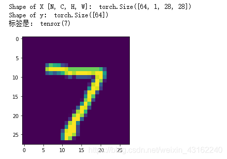
    print("Shape of X [N, C, H, W]: ", X.shape)
    print("Shape of y: ", y.shape)
    # 这里X是64张图片，X[0]表示第一张图片，X[0][0]表示第一个通道，plt.imshow是一个内置函数，可以打印图片的。
    plt.imshow(X[0][0])  
    print("标签是：",y[0])  # 这里y有64个标签，y[0]表示第一张图的标签
    break

The output is as follows:

Create a neural network model

    After the data is ready, the model can be created and ready for training.
    The model created here uses pytorch's built-in function nn.Sequential and nn.Conv2d, nn.MaxPool2d, nn.Flatten, nn.Linear, nn.ReLU. Here Sequential is used to combine each layer; Flatten is to flatten the two-dimensional image 28*28 into a 784-sized vector; Linear represents a linear classifier; relu represents an activation function.

# Define model
model = nn.Sequential(
                    nn.Conv2d(1, 64, 3, 1, 1),
                    nn.ReLU(),
                    nn.MaxPool2d(2, 2),
                    nn.Conv2d(64, 128, 3, 1, 1),
                    nn.ReLU(),
                    nn.MaxPool2d(2, 2),
                    nn.Flatten(),
                    nn.Linear(7*7*128, 1024),
                    nn.ReLU(),
                    nn.Dropout(p = 0.3),
                    nn.Linear(1024, 10))

training model

# 定义超参数，迭代轮数，学习率
iter_times=20
learningrate=1e-3

# 定义损失函数，这里直接用torch内置的交叉熵损失函数
loss_fn = nn.CrossEntropyLoss()
# 定义优化器，这里直接用torch内置的SGD梯度下降
optimizer = torch.optim.SGD(model.parameters(), lr=learningrate)

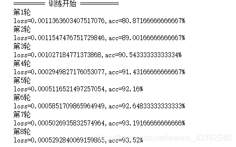
print("======= 开始训练 ======")
size = len(train_dataloader.dataset)
for i in range(iter_times):
	correct = 0
    for X, y in train_dataloader:
		# model是之前定义的模型，然后model(X)表示X经过模型得到的预测结果
		# loss_fn是torch内置计算损失的函数，输入是预测值与对应的实际标签。
        pred = model(X)
        loss = loss_fn(pred, y)

        # 下面三个是神经网络反向传播标准化流程，分别是梯度置零，反向传播计算梯度，参数更新
        optimizer.zero_grad()
        loss.backward()
        optimizer.step()
        
		# 通过预测值与标签计算这一个批次的准确率
		# 这个准确率是训练集的准确率，可以判断模型学习的好坏，但是无法判断泛化性。
        correct += (pred.argmax(1) == y).type(torch.float).sum().item()
     
    # 每轮迭代之后打印一下损失，这里print里面用的是"".format()方式。
    loss = loss.item()
    print("第{}轮".format(i+1))
    print("loss={},acc={}%".format(loss,100*correct/size))

The output here sees that the accuracy rate on the training set is constantly increasing, indicating that the model is well trained.

validation model

size = len(test_dataloader.dataset)
model.eval()  # .eval避免测试集也被训练了，以下mo_grad也是避免计算梯度，加快测试速度
correct = 0
with torch.no_grad():
    for X, y in test_dataloader:
        pred = model(X)
        correct += (pred.argmax(1) == y).type(torch.float).sum().item()
correct /= size   # 除以累加次数计算平均准确率
print("Accuracy:{}%".format(100*correct))