pytorch (2): color picture recognition

1 Development environment

Computer system: Windows 10

Compiler: Jupter Lab

Locale: Python 3.8

Deep learning environment: Pytorch

2 Preliminary preparation

2.1 Set GPU

        Since the computer graphics card used in the experiment is an integrated graphics card (intel(r) UHD graphics), the GPU cannot be used.

# 设置GPU(没有GPU则为CPU)
import torch
import torch.nn as nn
import matplotlib.pyplot as plt
import torchvision

device = torch.device("cuda" if torch.cuda.is_available() else "cpu")

print('device', device)

2.2 Import data

2.2.1 Download data

        Use torchvision.datasets..CIFAR10 to download the CIFAR10 dataset, and divide the training set and test set.

        If the CIFAR10 dataset has been downloaded locally, read it directly from the local (by adjusting the parameter download = False)

(1) Function prototype

torchvision.datasets.CIFAR10(root, train=True, transform=None, target_transform=None, download=False)

(2) Parameter description

root (string): data address

train (string) : True = training set, False = test set

download (bool,optional) : If True, download the dataset from the Internet and put the dataset in the root directory.

transform (callable, optional): The parameter here selects a data transformation function you want, and directly completes the data transformation

target_transform (callable, optional) : A function/transform that takes a target and transforms it.

(3) Experiment code

import os

ROOT_FOLDER = 'data'
CIFAR10_FOLDER = os.path.join(ROOT_FOLDER, 'cifar-10-batches-py')
if not os.path.exists(CIFAR10_FOLDER) or not os.path.isdir(CIFAR10_FOLDER):
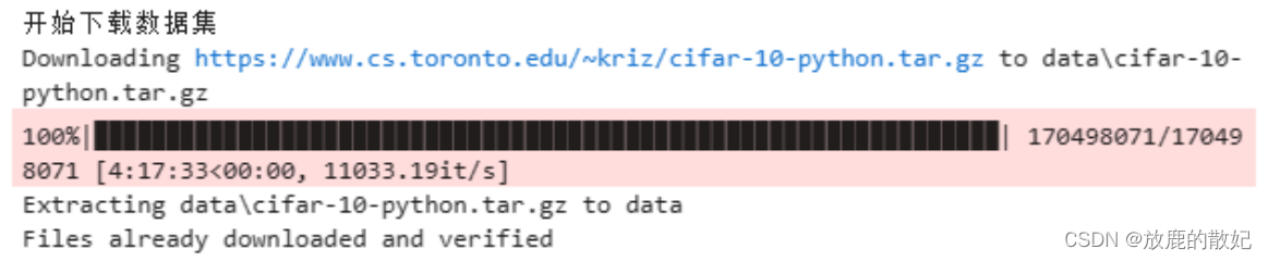
    print('开始下载数据集')
    # 下载训练集
    train_ds = torchvision.datasets.CIFAR10(ROOT_FOLDER, 
                                            train=True, 
                                            transform=torchvision.transforms.ToTensor(), # 将数据类型转化为Tensor
                                            download=True)
    # 下载测试集
    test_ds  = torchvision.datasets.CIFAR10(ROOT_FOLDER, 
                                            train=False, 
                                            transform=torchvision.transforms.ToTensor(), # 将数据类型转化为Tensor
                                            download=True)
else:
    print('数据集已下载 直接读取')
    # 读取已下载的训练集
    train_ds = torchvision.datasets.CIFAR10(ROOT_FOLDER, 
                                            train=True, 
                                            transform=torchvision.transforms.ToTensor(), # 将数据类型转化为Tensor
                                            download=False)
    # 读取已下载的测试集
    test_ds  = torchvision.datasets.CIFAR10(ROOT_FOLDER, 
                                            train=False, 
                                            transform=torchvision.transforms.ToTensor(), # 将数据类型转化为Tensor
                                            download=False)

        The execution result is as follows:

        After running, download the data package under the data folder and convert the data set directly into Tensor

2.2.2 Loading data

        Use torch.utils.data.DataLoader to load data, and set batch_size=32, so the shape of the final output image data is [32, 3, 32, 32].

batch_size = 32
# 从 train_ds 加载训练集
train_dl = torch.utils.data.DataLoader(train_ds, 
                                       batch_size=batch_size, 
                                       shuffle=True)
# 从 test_ds 加载测试集
test_dl  = torch.utils.data.DataLoader(test_ds, 
                                       batch_size=batch_size)

# 取一个批次查看数据格式
# 数据的shape为：[batch_size, channel, height, weight]
# 其中batch_size为自己设定，channel，height和weight分别是图片的通道数，高度和宽度。
imgs, labels = next(iter(train_dl))
print('Image shape: ', imgs.shape, '\n')
# torch.Size([32, 3, 32, 32])  # 所有数据集中的图像都是32*32的RGB图

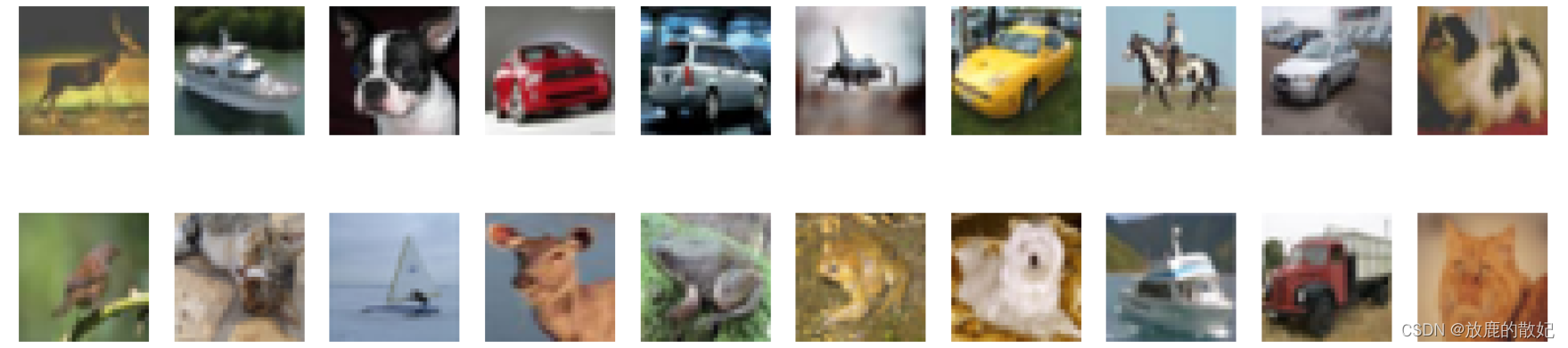
2.3 Data Visualization

import numpy as np

 # 指定图片大小，图像大小为20宽、5高的绘图(单位为英寸inch)
plt.figure('Data Visualization', figsize=(20, 5)) 
for i, imgs in enumerate(imgs[:20]):
    # 维度顺序调整 [3, 32, 32]->[32, 32, 3]
    npimg = imgs.numpy().transpose((1, 2, 0))
    # 将整个figure分成2行10列，绘制第i+1个子图。
    plt.subplot(2, 10, i+1)
    plt.imshow(npimg, cmap=plt.cm.binary)
    plt.axis('off')

3 Build a simple CNN network

        For a general CNN network, it is composed of a feature extraction network and a classification network. The feature extraction network is used to extract the features of the picture, and the classification network is used to classify the picture.

3.1 torch.nn.Conv2d()

        Conv2d is a convolutional layer used to extract the features of pictures.

(1) Function prototype

torch.nn.Conv2d(in_channels, out_channels, kernel_size, stride=1, padding=0, dilation=1, groups=1, bias=True, padding_mode=‘zeros’, device=None, dtype=None)

1. Parameter Description

in_channels (int): the number of channels in the input image

out_channels (int): the number of channels produced by the convolution

kernel_size (int or tuple): the size of the convolution kernel

stride (int or tuple, optional): The stride of the convolution. The default value is 1

padding (int, tuple or str, optional): Padding added to all four sides of the input. The default value is 0

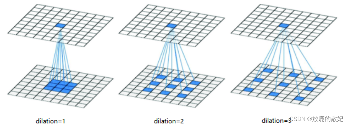
dilation( int or tuple , optional ): dilation operation, control the spacing of kernel points (convolution kernel points), the default value is 1

padding_mode (string, optional): 'zeros', 'reflect', 'replicate' or 'circular'. The default is 'zeros'

        The diagram about dilation is shown in the figure below:

3.2 torch.nn.Linear()

        Linear is a fully connected layer that can function as a feature extractor, and the fully connected layer of the last layer can also be considered as an output layer.

(1) Function prototype

torch.nn.Linear(in_features, out_features, bias=True, device=None, dtype=None)

(2) Parameter description

in_features: the size of each input sample

out_features: the size of each output sample

3.3  torch.nn.MaxPool2d()

        MaxPool2d is a pooling layer that performs downsampling and represents image features with a higher level of abstraction.

(1) Function prototype:

torch.nn.MaxPool2d(kernel_size, stride=None, padding=0, dilation=1, return_indices=False, ceil_mode=False)

(2) Parameter description:

kernel_size: the maximum window size

stride: the stride of the window, the default value is kernel_size

padding: padding value, default is 0

dilation: A parameter that controls the stride of elements in the window

3.4 CNN network construction

3.4.1 Code

import torch.nn.functional as F

num_classes = 10  # 图片的类别数

class Model(nn.Module):
    def __init__(self):
        super().__init__()
        # 特征提取网络
        self.conv1 = nn.Conv2d(3, 64, kernel_size=3)   # 第一层卷积,卷积核大小为3*3
        self.pool1 = nn.MaxPool2d(kernel_size=2)       # 设置池化层,池化核大小为2*2
        self.drop1 = nn.Dropout(p=0.15)
        self.conv2 = nn.Conv2d(64, 64, kernel_size=3)  # 第二层卷积,卷积核大小为3*3   
        self.pool2 = nn.MaxPool2d(kernel_size=2)       # 设置池化层,池化核大小为2*2
        self.drop2 = nn.Dropout(p=0.15)
        self.conv3 = nn.Conv2d(64, 128, kernel_size=3) # 第三层卷积,卷积核大小为3*3   
        self.pool3 = nn.MaxPool2d(kernel_size=2)       # 设置池化层,池化核大小为2*2
        self.drop3 = nn.Dropout(p=0.15)
        
        # 分类网络
        self.fc1 = nn.Linear(512, 256)
        self.fc2 = nn.Linear(256, num_classes)
    
    # 前向传播
    def forward(self, x):
        x = self.drop1(self.pool1(F.relu(self.conv1(x))))     
        x = self.drop2(self.pool2(F.relu(self.conv2(x))))
        x = self.drop3(self.pool3(F.relu(self.conv3(x))))
        
        x = torch.flatten(x, start_dim=1)
        
        x = F.relu(self.fc1(x))
        x = self.fc2(x)
        
        return x

3.4.2 Network data shape derivation

(1) Convolution layer shape calculation

        The calculation formula of the convolutional layer output shape size (O*O):

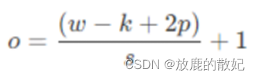
        Among them, w -- input data size (w*w)

      k -- convolution kernel size (k*k)

      s -- the step size

      p -- padding size (padding)

(2) Pooling layer shape calculation

        Pooling layer output shape size ([N,C,Hout,Wout] or [C,Hout,Wout], input data shape is [N,C,Hin,Win] or [C,Hin,Win]) calculation formula:

 

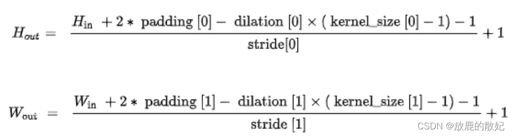
        Among them, kernel_size: pooling window size

      stride: the step size of the window, the default value is kernel_size

      padding: padding value, default is 0

      dilation: the parameter to control the stride of elements in the window, the default is 1      

(3) Network shape

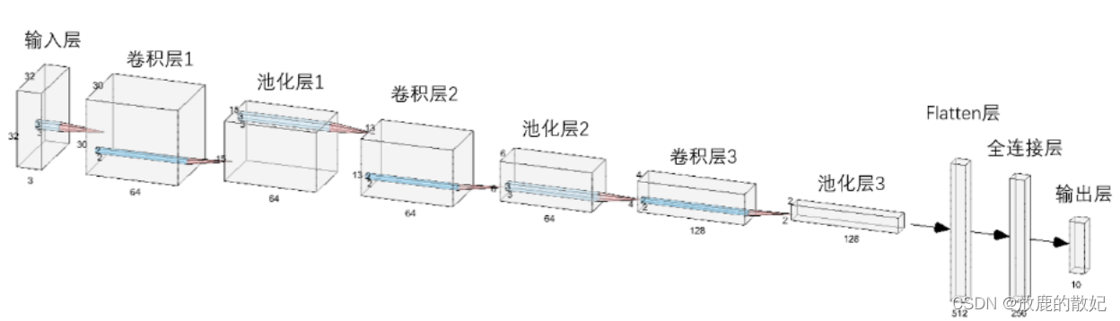
        According to the formulas in (1) and (2) and the settings of the parameters of each layer in the code, the size of each layer can be deduced as:

[3, 32, 32] (input data) -->

[64, 30, 30] （con1）--> [64, 15, 15] （pool1）-->

[64, 13, 13] （con2）--> [64, 6, 6] （pool2）-->

[128, 4, 4] （con3）--> [128, 2, 2] （pool1）-->

[3, 30, 30] （con1）--> [3, 15, 15] （pool1）-->

[512]（fc1）-> [256] （fc2）-->

[10] (output layer, num_class)

        The entire network structure is shown in the figure below:

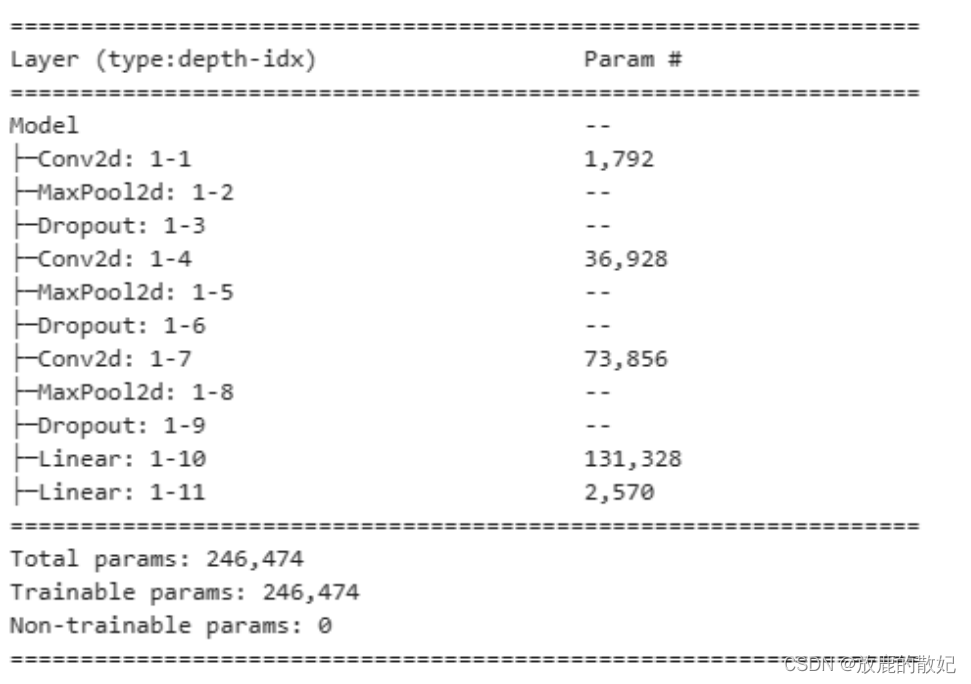
 3.4.3 Load and print the model

from torchinfo import summary
# 将模型转移到GPU中,但我的PC只能将模型运行在CPU中
model = Model().to(device)

summary(model)

The output is as follows:

3.4.4 Model packaging

        You can use torch.nn.Sequential to package the model, and the structure printing is clearer.

class ModelS(nn.Module):
    def __init__(self):
        super(ModelS, self).__init__()
        self.conv1=nn.Sequential(
            nn.Conv2d(3, 64, kernel_size=3, padding=0),# 64*30*30
            nn.ReLU(),
            nn.MaxPool2d(2),  #高宽减半 64*15*15
            nn.Dropout(0.15)
        )
        self.conv2=nn.Sequential(
            nn.Conv2d(64, 64, kernel_size=3, padding=0), # 64*13*13
            nn.ReLU(),
            nn.MaxPool2d(2),  #高宽减半 64*6*6
            nn.Dropout(0.15)
        )
        self.conv3=nn.Sequential(
            nn.Conv2d(64, 128, kernel_size=3, padding=0), # 128*4*4
            nn.ReLU(),
            nn.MaxPool2d(2),  #高宽减半 128*2*2
            nn.Dropout(0.15)
        )
        self.fc=nn.Sequential(
            nn.Linear(128*2*2, 256),
            nn.ReLU(), 
            nn.Linear(256, num_classes)
        )
    
    def forward(self, x):
       batch_size = x.size(0)
       x = self.conv1(x)  # 卷积-激活-池化-Dropout
       x = self.conv2(x)  # 卷积-激活-池化-Dropout
       x = self.conv3(x)  # 卷积-激活-池化-Dropout
       x = x.view(batch_size, -1)  # flatten 变成全连接网络需要的输入 
       x = self.fc(x)
       
       return x


model_s = ModelS().to(device)

summary(model_s)

4 training model 

4.1 Setting hyperparameters

loss_fn    = nn.CrossEntropyLoss() # 创建损失函数
learn_rate = 1e-2 # 学习率
opt        = torch.optim.SGD(model.parameters(),lr=learn_rate)

4.2 Write the training function

4.2.1 optimizer.zero_grad()

        This function traverses all the parameters of the model, cuts off the backpropagation gradient flow through the built-in method, and then sets the gradient value of each parameter to 0, that is, the previous gradient record is cleared.

4.2.2 loss.backward()

        PyTorch's backpropagation (tensor.backward()) is implemented through the autograd package, which automatically calculates its corresponding gradient based on the mathematical operations performed by the tensor.

        Specifically, torch.tensor is the basic class of the autograd package. If you set tensor's requires_grads to True, it will start tracking all operations on this tensor. If you use tensor.backward() after the operation, all gradients It will be calculated automatically, and the gradient of the tensor will be accumulated in its .grad attribute.

        More specifically, the loss function loss is obtained by a series of calculations for all weights w of the model. If the requires_grads of a certain w is True, then the .grad_fn attribute of all upper layer parameters of w (the weight w of the subsequent layer) will be The corresponding operation is saved, and then after using loss.backward(), each gradient value will be calculated through layer-by-layer backpropagation, and saved to the .grad attribute of w.

        If tensor.backward() is not performed, the gradient value will be None, so loss.backward() should be written before optimizer.step().

4.2.3 optimizer.step()

        The function of the step() function is to perform an optimization step and update the value of the parameter through the gradient descent method. Because the gradient descent is based on the gradient, the loss.backward() function should be executed to calculate the gradient before the optimizer.step() function is executed.

Note: The optimizer is only responsible for optimization through gradient descent, not for generating gradients, which are generated by the tensor.backward() method.

4.2.4 Training function code

# 训练循环
def train(dataloader, model, loss_fn, optimizer):
    size = len(dataloader.dataset)  # 训练集的大小
    num_batches = len(dataloader)   # 批次数目

    train_loss, train_acc = 0, 0  # 初始化训练损失和正确率
    
    for X, y in dataloader:  # 获取图片及其标签
        X, y = X.to(device), y.to(device)
        
        # 计算预测误差
        pred = model(X)          # 网络输出
        loss = loss_fn(pred, y)  # 计算网络输出和真实值之间的差距，y为真实值，计算二者差值即为损失
        
        # 反向传播
        optimizer.zero_grad()  # grad属性归零
        loss.backward()        # 反向传播
        optimizer.step()       # 每一步自动更新
        
        # 记录acc与loss
        train_acc  += (pred.argmax(1) == y).type(torch.float).sum().item()
        train_loss += loss.item()
            
    train_acc  /= size
    train_loss /= num_batches

    return train_acc, train_loss

4.3 Writing test functions

        The test function is roughly the same as the training function, but since the network weights are not updated by gradient descent, there is no need to pass in the optimizer.

def test (dataloader, model, loss_fn):
    size        = len(dataloader.dataset)  # 测试集的大小
    num_batches = len(dataloader)          # 批次数目
    test_loss, test_acc = 0, 0
    
    # 当不进行训练时，停止梯度更新，节省计算内存消耗
    with torch.no_grad():
        for imgs, target in dataloader:
            imgs, target = imgs.to(device), target.to(device)
            
            # 计算loss
            target_pred = model(imgs)
            loss        = loss_fn(target_pred, target)
            
            test_loss += loss.item()
            test_acc  += (target_pred.argmax(1) == target).type(torch.float).sum().item()

    test_acc  /= size
    test_loss /= num_batches

    return test_acc, test_loss

4.4 Formal training

4.4.1  model.train()

        The role of model.train() is to enable Batch Normalization and Dropout.

        If there are BN layers (Batch Normalization) and Dropout in the model, you need to add model.train() during training. model.train() is to ensure that the BN layer can use the mean and variance of each batch of data. For Dropout, model.train() randomly selects a part of the network connection to train and update parameters.

4.4.2 model.eval()

        The function of model.eval() is not to enable Batch Normalization and Dropout.

        If there are BN layers (Batch Normalization) and Dropout in the model, add model.eval() during testing. model.eval() is to ensure that the BN layer can use the mean and variance of all training data, that is, to ensure that the mean and variance of the BN layer remain unchanged during the test. For Dropout, model.eval() utilizes all network connections, that is, does not randomly discard neurons.

        After training the train samples, the generated model model is used to test the samples. Before model(test), you need to add model.eval(), otherwise, if there is input data, it will change the weight even if it is not trained. This is the nature of the BN layer and Dropout in the model.

4.4.3 Training code

import time

epochs     = 30
train_loss = []
train_acc  = []
test_loss  = []
test_acc   = []

print('\nStart training...')
for epoch in range(epochs):
    model.train()
    epoch_train_acc, epoch_train_loss = train(train_dl, model, loss_fn, opt)
    
    model.eval()
    epoch_test_acc, epoch_test_loss = test(test_dl, model, loss_fn)
    
    train_acc.append(epoch_train_acc)
    train_loss.append(epoch_train_loss)
    test_acc.append(epoch_test_acc)
    test_loss.append(epoch_test_loss)
    
    template = ('Epoch:{:2d}, Train_acc:{:.1f}%, Train_loss:{:.3f}, Test_acc:{:.1f}%，Test_loss:{:.3f}')
    print(time.strftime('[%Y-%m-%d %H:%M:%S]'), template.format(epoch+1, epoch_train_acc*100, epoch_train_loss, epoch_test_acc*100, epoch_test_loss))
print('Done')

        The following is the training output:

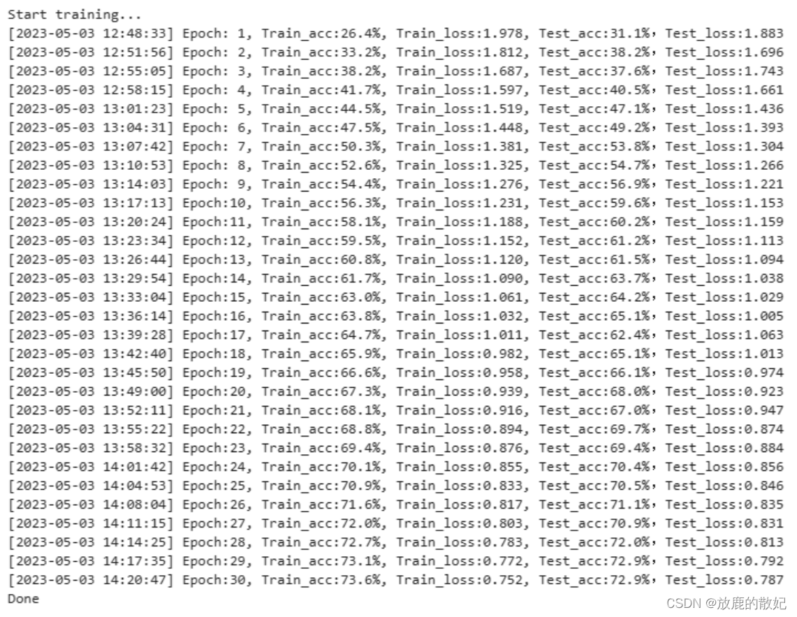
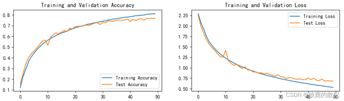
        In the final result, the accuracy rate of the training set reached 73.6%, and the accuracy rate of the test set reached 72.9%, and the loss still has a downward trend, indicating that it is currently in a state of underfitting and needs to continue training.

        Change the number of training times to 50 times and retrain. The accuracy rate of the training set reaches 81.2%, and the accuracy rate of the test set reaches 76.9%, but it is still in an underfitting state and needs to continue training.

 5 Prediction and Results Visualization

import matplotlib.pyplot as plt
#隐藏警告
import warnings
warnings.filterwarnings("ignore")               #忽略警告信息
plt.rcParams['font.sans-serif']    = ['SimHei'] # 用来正常显示中文标签
plt.rcParams['axes.unicode_minus'] = False      # 用来正常显示负号
plt.rcParams['figure.dpi']         = 100        #分辨率

epochs_range = range(epochs)

plt.figure('Result Visualization', figsize=(12, 3))
plt.subplot(1, 2, 1)

plt.plot(epochs_range, train_acc, label='Training Accuracy')
plt.plot(epochs_range, test_acc, label='Test Accuracy')
plt.legend(loc='lower right')
plt.title('Training and Validation Accuracy')

plt.subplot(1, 2, 2)
plt.plot(epochs_range, train_loss, label='Training Loss')
plt.plot(epochs_range, test_loss, label='Test Loss')
plt.legend(loc='upper right')
plt.title('Training and Validation Loss')
plt.show()

6 Summary

        Compared with the previous minist handwritten digit recognition project, this section is not much different, except that the data set and network are slightly more complicated (a set of Conv2d+MaxPool2d+Dropout is added), basically there is no big change.