Introduction to Deep Learning Basics [7]: Commonly used normalization algorithms, hierarchical normalization algorithms, normalization and standardization are different from connections, and application case scenario analysis.

[Introduction to advanced deep learning] must-see series, including activation function, optimization strategy, loss function, model tuning, normalization algorithm, convolution model, sequence model, pre-training model, adversarial neural network, etc.

The column introduces in detail: [Introduction to advanced deep learning] must-see series, including activation function, optimization strategy, loss function, model tuning, normalization algorithm, convolution model, sequence model, pre-training model, adversarial neural network, etc.

This column is mainly to facilitate beginners to quickly grasp relevant knowledge. Disclaimer: Some projects are online classic projects for everyone to learn quickly, and practical links will be added in the future (competitions, papers, practical applications, etc.)

Column Subscription: Deep Learning Introduction to Advanced Columns

1. Normalized basic knowledge points

1.1 Normalization

Normalization is a data processing method that can limit the data to a fixed range after processing.

Normalization exists in two forms,

• One is to process the number as a decimal between [0, 1] under normal circumstances, the purpose of which is to facilitate the subsequent data processing . For example, in image processing, the image will be normalized from [0, 255] to [0, 1], so that the information storage of the image itself will not be changed, and the subsequent network processing will be accelerated.
• In other cases, the data can also be processed between [-1, 1], or within other fixed ranges. The other is to convert a dimensioned expression into a dimensionless expression through normalization.

So what is dimension, and why do we need to convert dimensionality into dimensionless? Give an example. When we are predicting housing prices, the collected data, such as the area of ​​the house, the number of rooms, the distance to the subway station, the air quality near the house, etc., are all dimensions, and their corresponding dimensional units They are square meters, number, meters, AQI, etc. The difference in these dimensional units makes the data not comparable. At the same time, for different dimensions, the order of magnitude of the data is also different. For example, the distance from a house to a subway station can be thousands of meters, but the number of rooms in a house is generally only a few. After normalization processing, not only can the influence of dimension be eliminated, but also all data can be normalized to the same magnitude, so as to solve the comparability problem among data .

• Normalization can convert dimensionality into dimensionless, and at the same time normalize data to the same magnitude to solve the problem of comparability between data. In a regression model, inconsistent dimensions of the independent variables can lead to uninterpretable or misinterpreted regression coefficients. In KNN, Kmeans and other algorithms that need to perform distance calculations, the different magnitudes of dimensions may cause features with larger magnitudes to dominate in distance calculations, thereby affecting the learning results.

• After the data is normalized, the process of seeking the optimal solution will become smoother, and the optimal solution can be converged more quickly. For details, please refer to 3. Why normalization can improve the speed of solving the optimal solution.

1.2 Normalization improves the speed of solving the optimal solution

We mentioned an example of predicting housing prices. Suppose the independent variables are only the distance x1 from the house to the subway station and the number of rooms in the house x2. The dependent variable is the housing price. The prediction formula and loss function are respectively

$\begin{array}{l}y=i_1{x}_1+i_2{x}_2\\ J=(i_1{x}_1+i_2{x}_2-y_{label}{)}^2\end{array}$

When not normalized, the distance from the house to the subway station ranges from 0 to 5000, while the number of rooms ranges from 0 to 10. Suppose x1=1000, x2=3, then the formula of the loss function can be written as:

$J={\left(1000i_1+3i_2-y_{label}\right)}^2$

The process of seeking the optimal solution for this loss function can be visualized as the following figure: Figure 1: The contour line of the loss function, Figure 1 (left) is when it is not normalized, and Figure 1 (right) is normalized

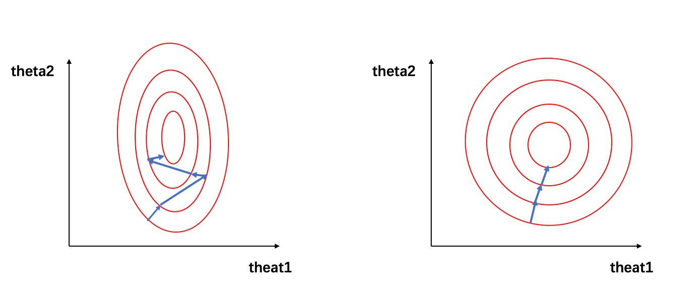
In Figure 1, the red ellipse on the left represents the contour of the loss function before normalization, the blue line segment represents the update of the gradient, and the direction of the arrow represents the direction of the gradient update. The process of seeking the optimal solution is the process of gradient update, and its update direction is perpendicular to the climbing line. Due to the large difference between the magnitudes of x1 and x2, the contour line of the loss function appears as a thin and narrow ellipse. Therefore, as shown in Figure 1 (left), the narrow ellipse will make the gradient descent process appear in a zigzag, resulting in a slow gradient descent.

When the data is normalized, $x_1^{{}^{\prime }}=\frac{1000-0}{5000-0}=0.2,x_2^{{}^{\prime }}=\frac{3-0}{10-0}=0.3,$ , then the formula of the loss function can be written as:

$J(x)={\left(0.2i_1+0.3i_2-y_{label}\right)}^2$

We can see that the normalized data belong to the same magnitude, and the contour line of the loss function presents a chunky ellipse (as shown in Figure 1 (right)), and the process of solving the optimal solution becomes easier Fast and gentle, so faster convergence can be obtained when solving by gradient descent.

1.3 Normalization type

1.3.1 Min-max normalization (Rescaling)：

$x^{{}^{\prime }}=\frac{x-min(x)}{max(x)-min(x)}$

The normalized data range is [0, 1], where min(x) and max(x) find the minimum and maximum values ​​of the sample data respectively.

1.3.2 Mean normalization：

$x^{{}^{\prime }}=\frac{x-mean(x)}{max(x)-min\left(x\right)}$

1.3.3 Z-score normalization (Standardization): standardization

$x^{{}^{\prime }}=\frac{x-}{p}$

The normalized data range is a set of real numbers, where μ and σ are the mean and standard deviation of the sample data, respectively.

1.3.4 Nonlinear normalization:

• Log normalization:
  $x^{{}^{\prime }}=\frac{\lg x}{\lg max\left(x\right)}$

• The arctangent function is normalized:

$x^{{}^{\prime }}=\arctan \left(x\right)\ast \frac{2}{Pi}$

The normalized data range is [-1, 1]

• Demical Point Normalization:

$x^{{}^{\prime }}=\frac{x}{10^j}$

The normalized data range is [-1, 1], j is to make $max(|x^{\prime }|)<The\; smallest\; integer\; of\; 1$ .

1.4 Conditions of use for different normalizations

1. Min-max normalization and mean normalization are suitable for use when the maximum and minimum values ​​are clearly unchanged . For example, in image processing, the gray value is limited to the range of [0, 255], you can use min-max normalization One process it to [0, 1]. When the maximum and minimum values ​​are not clear, whenever new data is added, the maximum or minimum value may be changed, resulting in unstable normalization results and unstable subsequent use effects. At the same time, the data needs to be relatively stable. If there are too large or too small outliers, the effect of min-max normalization and mean normalization will not be very good. If there are strict requirements on the range of processed data, min-max normalization or mean normalization should also be used.

2. Z-score normalization can also be called standardization , and the processed data is distributed with a mean of 0 and a standard deviation of 1. Standardization can be used when there are outliers in the data and the maximum and minimum values ​​are not fixed . Standardization changes the state distribution of the data, but not the kind of distribution. In particular, z-score normalization is often used in neural networks, and we will introduce it in detail in subsequent articles.

3. Nonlinear normalization is usually used in scenarios where the data is highly differentiated , and sometimes it is necessary to map the original value through some mathematical functions, such as logarithm, arctangent, etc.

When searching for information, I saw many articles that said: "In classification and clustering algorithms, when distance is needed to measure similarity, z-score normalization, that is, standardization, is better than normalization , but there is not enough technical support for this point of view. Therefore, I selected the KNN classification network to search for related papers. In the paper Comparative Analysis of KNN Algorithm using Various Normalization Techniques [1], in the case of different K values , respectively perform min-max normalization and z-score normalization on the same data, and the results obtained are shown in the figure below: Figure 2: For different K values, the prediction accuracy under different normalization methods for the same data set Spend

It can be seen that, at least for KNN classification problems, the choice of z-score normalization and min-max normalization will be affected by the data set and K value. For other classification and clustering algorithms, which normalization The method of integration is better still to be verified. The best way to choose is to conduct experiments and choose the one that can make the model more accurate under the current experimental conditions.

1.5 The connection and difference between normalization and standardization

When it comes to normalization and standardization, there may be some conceptual confusion. We all know that normalization refers to normalization, and standardization refers to standardization . However, according to the definition of feature scaling method on wiki, standardization is actually z-score normalization, also That is to say, standardization is actually a kind of normalization. In general, we will refer to z-score normalization as standardization, and min-max normalization as normalization for short. In the following, we also refer to z-score normalization by normalization and min-max normalization by normalization.

In fact, normalization and standardization are essentially linear transformations. In 4. Normalization type, we mentioned the formula of normalization and standardization. For the formula of normalization, when the data is given, a=max(x)−min(x), b =min(x), the normalized formula can be transformed into:

$x^{{}^{\prime }}=\frac{x-b}{a}=\frac{x}{a}-\frac{b}{a}=\frac{x}{a}-c$

The normalized formula is similar to the deformed normalization, where μ and σ can be regarded as constants when the data is given. Therefore, the normalized deformation is similar to the normalized one, which can be regarded as scaling x by a ratio, and then performing a translation of c units. It can be seen that the essence of normalization and standardization is a linear transformation, and they will not change the original numerical order of the data due to the processing of the data.

So what is the difference between normalization and standardization?

• Normalization does not change the state distribution of the data, but standardization changes the state distribution of the data;

• Normalization will limit the data to a specific range, such as [0, 1], but standardization will not. Standardization will only process the data as a mean of 0 and a standard deviation of 1.

References:【1】Comparative Analysis of KNN Algorithm using Various Normalization Techniques；Amit Pandey，Achin Jain.

2. Layer normalization

The learning process of the neural network is essentially learning the distribution of data . If normalization is not performed, the distribution of each batch of training data is different.

• From a general perspective, the neural network needs to find a balance among these multiple distributions.
• From a small perspective, since the distribution of network input data in each layer is constantly changing, it will cause each layer of the network to find a balance point, and obviously the network becomes difficult to converge .
  Of course, we can normalize the input data (such as dividing the input image by 255), but this can only ensure that the data distribution of the input layer is the same, and it cannot guarantee that the input data distribution of each layer of the network is the same, so In the middle of the network, we also need to add normalization processing.

Definition of normalization: Data standardization (Normalization), also known as normalization, normalization is to limit the data to be processed within a certain range after being processed by a certain algorithm

2.1 Reasons for layer normalization

• The general batch normalization (Batch Normalization, BN) algorithm relies too much on the mini-batch data set and cannot be applied to online learning tasks (the number of samples contained in the mini-batch data set is 1 at this time). The effect of BN in the network (Recurrent neural network, RNN) is not obvious;
• RNN is mostly used for natural language processing tasks. The sentences input by the network in different training cycles often have different sentence lengths. When applying BN in RNN, the size of the mini-batch data set used in different time periods needs to be different, and the calculation is complicated. If a test sentence is longer than any sentence in the training set, the prediction performance of the RNN neural network will be severely biased during the test phase. If you change to use layer normalization, you can effectively avoid this problem.

Layer normalization: Neurons are normalized by calculating the mean and variance of all neurons in a layer on a training sample.

$$\begin{gathered} m\leftarrow \frac{1}{H}{\sum }_{i=1}^H{x}_i \\ p\leftarrow \sqrt{\frac{1}{H}{\sum }_{i=1}^H(x_i-m_D{)}^2+ϵ} \\ ⋮ \\ y=f(\frac{g}{p}(x-m)+b) \end{gathered}$$

Related parameter meanings:

• x : vector representation of neurons in this layer

• H : the number of hidden neurons in the layer

• ϵ : add small value to variance to prevent division by zero

• g: rescaling parameters (trainable), new data with g2 as variance

• b: re-translation parameters (trainable), the new data is biased by b

• f: activation function

Algorithm role

1. Accelerate the convergence speed of network training. In a deep neural network, if the data distribution of each layer is different, it will make the network very difficult to converge and train (as mentioned in the review, it is difficult to find a balance point among multiple data distributions), and each If the distribution of layer data is the same, the convergence speed during training will be greatly improved.

To control gradient explosion and prevent gradient disappearance, our usual way of gradient transfer is from deep neurons to shallow layers. If f'i and O'i are used to represent the activation layer derivative and output derivative corresponding to the i-th layer respectively, then for H Layer neural network, the derivative of the first layer $F_1^{\prime }={\prod }_{i=1}^H{f}_i^{\prime }\ast O_i^{\prime }$, between to $f_i^{\prime }\ast O_i^{\prime }$Always greater than 1, such as $f_i^{\prime }\ast O_i^{\prime }=$In the case of$2$$f_i^{\prime }\ast O_i^{\prime }$Heng Xiao Yu 1, like $f_i^{\prime }\ast O_i^{\prime }=0.25$ leads to an exponential decline in the result, the phenomenon of gradient disappearance occurs, and the gradient of the underlying neuron is almost 0. After using the normalization algorithm, f_i'*O_i'$f_i^{\prime }\ast O_i^{\prime }$The result of will not be too large or too small, which is conducive to controlling the propagation of gradients.

In the Fly Paddle frame case as follows:

paddle.nn.LayerNorm(normalized_shape, epsilon=1e-05, weight_attr=None, bias_attr=None, name=None);

This interface is used to construct a callable object of the LayerNorm class

The meaning of the core parameters:

• normalized_shape (int|list|tuple) – Which dimensions are expected to be transformed. If an integer, the last dimension is normalized.

• epsilon (float, optional) - corresponds to ϵ - the value to add to the denominator for numerical stability. Default: 1e-05

2.2 Application Cases

import paddle
import numpy as np

np.random.seed(123)
x_data = np.random.random(size=(2, 2, 2, 3)).astype('float32')
x = paddle.to_tensor(x_data)
layer_norm = paddle.nn.LayerNorm(x_data.shape[1:])
layer_norm_out = layer_norm(x)

print(layer_norm_out)

# input
# Tensor(shape=[2, 2, 2, 3], dtype=float32, place=CPUPlace, stop_gradient=True,
#        [[[[0.69646919, 0.28613934, 0.22685145],
#           [0.55131477, 0.71946895, 0.42310646]],

#          [[0.98076421, 0.68482971, 0.48093191],
#           [0.39211753, 0.34317800, 0.72904968]]],


#         [[[0.43857226, 0.05967790, 0.39804426],
#           [0.73799539, 0.18249173, 0.17545176]],

#          [[0.53155136, 0.53182757, 0.63440096],
#           [0.84943181, 0.72445530, 0.61102349]]]])

# output:
# Tensor(shape=[2, 2, 2, 3], dtype=float32, place=CPUPlace, stop_gradient=True,
#        [[[[ 0.71878898, -1.20117974, -1.47859287],
#           [ 0.03959895,  0.82640684, -0.56029880]],

#          [[ 2.04902983,  0.66432685, -0.28972855],
#           [-0.70529866, -0.93429095,  0.87123591]]],


#         [[[-0.21512909, -1.81323946, -0.38606915],
#           [ 1.04778552, -1.29523218, -1.32492554]],

#          [[ 0.17704056,  0.17820556,  0.61084229],
#           [ 1.51780486,  0.99067575,  0.51224011]]]])

For the general picture training set format is $(N,C,H,W)$ , in the LN transformation, we normalize the last three dimensions. Therefore, the input shape of the instance is the last three-dimensional x_data.shape[1:]. That is, we fixed each picture as a unit, and uniformly performed Z-score normalization on the pixel values ​​of all channels of each picture.

2.3 Application scenarios

The effect of layer normalization in the recurrent neural network RNN ​​is the most beneficial, and its performance is better than batch normalization, especially in the tasks of dynamic long sequences and small batches. For example, in the following tasks mentioned in the paper Layer Normalization:

1. Order embedding of images and language

2. Teaching machines to read and comprehend

3. Skip-thought向量（Skip-thought vectors）

4. Modeling binarized MNIST using DRAW (Modeling binarized MNIST using DRAW)

5. Handwriting sequence generation

6. Permutation invariant MNIST (Permutation invariant MNIST)

However, studies have shown that in the convolutional neural network, the LN will destroy the features learned by the convolution, causing the model to fail to converge. For the BN algorithm, based on the situation of different data, the data obtained by normalizing the same feature is even worse. It is easy to lose information, so in scenarios where both LN and BN can be applied, BN's performance is usually better.

Literature: Ba JL , Kiros JR , Hinton GE . Layer Normalization[J]. 2016.