YOLO those things [YOLOv1-YOLOv3 detailed explanation]

The detection model running on the GPU platform, commonly used backbones include VGG, ResNet, DarkNet , etc.
Detection models running on CPU platforms or edge devices, commonly used backbones are MobileNet, ShuffleNet, SqueezeNet , etc.

Neck : Integrate the features of different feature layers , integrate the rich positional information of the shallow layer and the rich semantic information of the deep layer, and improve the detection effect

Additional blocks：SPP，ASPP，RFB，SAM
Path-aggregation blocks：FPN，PAN，NAS-FPN，Fully-connected FPN，BiFPN，ASFF，SFAM

Heads : object localization and classification

Dense Prediction: Immediate one-stage method
- Anchor based: YOLO series, SSD, RetinaNet, RPN
- anchor free：CornerNet，CenterNet，MatrixNet，FCOS
Sparse Prediction: Immediate two-stage method
- anchor based：Faster R-CNN，R-FCN，Mask R-CNN
- anchor free：RepPoints

3. Target detection optimization techniques

3.1 Bag of freebies (BOF) - Improve detection accuracy without increasing inference time

data augmentation
1. Photometric Transform: Adjust Brightness, Contrast, Hue, Saturation and Noise
2. Geometric transformations: random scaling, cropping, flipping and rotating
3. Simulate target occlusion: random erase, CutOut, Hide and Seek, grid Mask
4. Image Fusion: MixUp, CutMix, Mosaic
5. HOWEVER
Loss function for bounding box regression
1. IOU Loss
2. GIOU Loss
3. DIOU Loss
4. CIOU Loss
Regularization
1. DropOut
2. DropConnect
3. DropBlock
Label Smoothing - Label Smoothing
Data Imbalance - Focal Loss

3.2 Bag of specials (BOS) —— Slightly increase the reasoning cost and bring great performance improvement

Enhanced receptive field
1. SPP
2. ASPP
3. RFB
feature fusion
1. Skip connection
2. FPN
3. SFAM
4. ASFF
5. BiFPN
Post-processing
1. NMS
2. soft NMS
3. DIOU NMS
attention module
1. Channel Attention (channel-wise) SE
2. Spatial attention (point-wise) SAM
activation function
1. LReLU (solve the case where the ReLU gradient is 0 when the input is less than 0)
2. PReLU (solve the case where the ReLU gradient is 0 when the input is less than 0)
3. ReLU6 (designed specifically for quantized networks)
4. hard-swish (designed specifically for quantized networks)
5. SELU (self-normalizing neural networks)
6. Swish (continuously differentiable activation function)
7. Mish (continuously differentiable activation function)

4. Target detection evaluation index

4.1 Speed index

The speed index is usually measured by inferring frames per second (FPS) (Frames Per Second) , which is greatly affected by hardware

4.2 Accuracy index

Target detection input image, output the rectangular coordinates of each target prediction frame in the image and the prediction confidence of each category, use the intersection and union ratio IOU to measure the coincidence degree of the prediction frame and the label frame, that is, whether the positioning of the prediction frame is accurate

According to the relationship with the labeled frame, a prediction frame can be divided into one of the following four categories, where the IOU threshold (generally 0.5) and confidence threshold (generally 0.2) are manually specified:

(1) Precision (accuracy rate) : The proportion of correct predictions in all prediction boxes reflects the accuracy of the model " not to mistake the background as a target"

(2) Recall (recall rate, recall rate) : The proportion of all labeled boxes that are correctly predicted reflects the sensitivity of the model to " do not let the target go as the background "

(3) Average Precision (AP for short) : Change the confidence threshold from 0-1, calculate the Precision and Recall corresponding to each confidence threshold, and draw a certain category of PR performance curve (P and R cannot be complete The prediction effect of the characterization network, it is hoped that P and R are larger values at the same time, that is, the area enclosed by the PR curve and the coordinate axis is larger), and the area enclosed by it is the AP of this category

Taking all categories of AP and different IOU thresholds, [email protected] and [email protected]:0.95 can be calculated respectively

[email protected] : When the IOU threshold is 0.5 , the average value of each category AP

[email protected]:0.95 : When the IOU threshold is takenwhen the 10 numbers increase from 0.5 to 0.95 , the average value of each category AP

5. YOLOv1

YOLO (You Only Look Once) is an object recognition and positioning algorithm based on a deep neural network - find an area in the picture where there is an object, and then identify which object is in the area. Its biggest feature is the speed of operation Soon , it can be used in real-time systems.

The first stage of two-stage target detection extracts potential candidate frames (Region Proposal), and the second stage uses a classifier to screen each candidate frame one by one. YOLO creatively combines the two stages of candidate regions and object recognition into one.

In fact, YOLO does not really remove the candidate area, but uses a predefined candidate area to divide the picture into 7 x 7=49 grids, and each grid allows to predict 2 borders (bounding box, containing a certain objects), a total of 49 x 2=98 bounding boxes.

5.1 YOLOv1 network structure

The size of the input image is 448 × 448 , after 24 convolutional layers and 2 fully connected layers, reshape operation, the output feature map size is 7 × 7 × 30 (PASCAL VOC data set).

The main idea:

Divide the input image into S*S grids, each grid is responsible for predicting the object centered in this grid
Each grid predicts B bounding boxes and their confidence levels, as well as C category probabilities
The bbox information (x, y, w, h) is the offset, width and height of the center position of the object relative to the grid position, all of which are normalized
- x, y are the coordinates of the center point of the bounding box relative to the grid point in the upper left corner of the grid cell
- w, h are the width and height of the bounding box relative to the entire image
Confidence reflects whether an object is contained, and the accuracy of the position if it is contained. Defined as Pr(Object)×IoU, where Pr(Object)∈{0,1}

5.2 Mapping relationship between input and output

5.3 Loss function

The center point of the bicycle in the figure is located in a grid of 4 rows and 3 columns, so the 30-dimensional vector of the position of 4 rows and 3 columns in the output tensor is shown in the upper right figure

Loss : The deviation between the actual output value of the network and the sample label value

Loss function:

5.4 Advantages and disadvantages of YOLOv1

Advantages of YOLOv1:

There is no need to extract candidate boxes and then classify and return candidate boxes one by one (single-stage). One forward inference can obtain bbox positioning and classification results, without complicated upstream and downstream processing work. End-to-end training optimization is fast and achieves real-time efficiency .
Migration generalizes well
The background error is small, and the whole image is directly selected for training, which can obtain global information (the RCNN series only processes the candidate frame area, so you can see the leopard in the tube)

YOLOv1 disadvantages:

Target positioning error is high and accuracy is insufficient
Low mAP, low accuracy, low Recall (lower than RCNN series) - "The target frame is not accurate, and the detection cannot be detected"

Cause Analysis:

The fully connected layer is used for final prediction, and the fully connected layer can be considered as a function acting on the features of the whole image. Target detection is a local prediction problem. It is contradictory to predict the position information of local objects with full image features.
YOLOv1 adopts a 7 x 7 grid division and predicts a total of 98 frames. It is difficult to achieve effective coverage of the targets appearing on the image , and the ability to detect all targets is poor.
Each grid unit of YOLOv1 only generates one prediction frame, and one grid can only predict one object , which causes YOLO-V1 to produce serious missed detection for densely distributed small targets.

6. YOLOv2

6.1 Improvement strategy

Although the detection speed of YOLOv1 is fast, the positioning is not accurate enough , and the recall rate is low . In order to improve the positioning accuracy and improve the recall rate, YOLOv2 proposes several improvement strategies based on YOLOv1 , as shown in the following figure:

1）Batch Normalization——increase of 4% mAP

In YOLOv2, a Batch Normalization (BN) layer is added after each convolutional layer, and the dropout layer is removed.
The Batch Normalization layer can have a certain regularization effect, which can improve the convergence speed of the model and prevent the model from overfitting

2) High Resolution Classifier (high resolution pre-trained classification network) - mAP increased by 4%

A general image classification network, pre-trained on ImageNet at a very small image resolution, e.g. 224 x 224
YOLOv1 network input is 448 x 448, switching from small resolution to large resolution, resulting in performance degradation
In order to adapt the network to the new resolution, YOLOv2 was first trained on ImageNet at 224 x 224, then fine-tuned on ImageNet for 10 epochs at 448 x 448, and finally fine-tuned on the target detection dataset at 448 x 448

3) Anchor Boxes - Recall increased by 7%, mAP decreased by 0.3%

YOLOv1 divides the picture into 7 x 7 grids, each grid predicts two bounding boxes, and the bbox with a large IOU of the ground truth is responsible for fitting the ground truth, and uses the fully connected layer to directly predict the bounding box, resulting in loss More spatial information , inaccurate positioning
YOLOv2 removes the fully connected layer in YOLOv1, uses an anchor mechanism similar to Faster R-CNN and SSD, uses Anchor Boxes to predict the bounding box , and binds several different scales and different lengths and widths to each position on the convolutional feature map. Compared with the predefined Anchor Boxes, each Anchor Boxes only needs to be fine-tuned in the original position, and the predicted offset is still the Anchor Box with the IOU larger than the ground truth is responsible for fitting the ground truth, and finally used for the predicted convolution The feature map is the corresponding bounding box position transformation parameters, confidence and target category probability
That is: which grid cell the center point of the manual annotation frame falls in, the Anchor with the largest IOU of the ground truth among the Anchors generated by the grid cell is responsible for prediction, and only needs to predict the offset relative to itself .
Motivation: Solve the problem of multiple targets in a grid (YOLOv1 can only detect one target in a grid)

Note ⚠️:

Tips1: YOLOv2 sets the feature map to an odd length and width

Reason: The feature map with odd length and width has a center cell. If there is a dominant large target in the image, its center point has a certain grid cell responsible for prediction, instead of four grid cells with even length and width to grab

Tips2: mAP decreases, Recall increases, and Precision decreases

Reason: YOLOv1 generates a maximum of 98 prediction frames, and YOLOv2 generates 845 prediction frames after adding Anchor. It can detect all the targets as much as possible, so the Recall is improved, but the proportion of useless frames in the 845 frames is also increased. Precision Reduced (the impact of reduced accuracy can be reduced by post-processing, so adding Anchor is worthwhile)

The 9 candidate frames generated by Faster RCNN's Anchor are "artificially" selected (the scale and aspect ratio parameters are set in advance, and generated according to certain rules), and YOLOv2 selects more reasonable candidate frames (it is difficult to establish a corresponding relationship with gt) Anchor is actually invalid), using the clustering (K-means) strategy (clustering the aspect ratio of the data set, experimentally clustering multiple anchor box groups with different numbers, and applying them to the model respectively to find out The set of anchor boxes that compromise between the complexity of the model and the high recall rate)
Advantages: Use the anchor mechanism to generate dense anchor boxes, so that the network can directly perform target classification and bounding box coordinate regression on this basis, effectively improve the recall ability of network targets, and significantly improve the detection of small targets
Disadvantages: There are a lot of redundant frames, and the targets in a picture are only limited. Setting a large number of anchor boxes for each anchor will generate a large number of background frames that do not contain targets at all, causing a serious imbalance between positive and negative samples.
Note: The prediction frame is based on Anchor, and is obtained by offsetting on the basis of Anchor

4) Dimension Clusters (the width and height of the Anchor Box are generated by clustering)

YOLOv2 uses the k-means clustering algorithm to cluster the bounding boxes in the training set, and selects the IOU value between boxes as the clustering index
The a priori box obtained by cluster analysis has a higher average IOU value than the manually selected a priori box, which makes the model easier to train and learn
Note: In the standard K-means clustering, the Euclidean metric is used as the distance criterion for clustering. Under this metric, the large frame tends to produce a larger error than the small frame. Therefore, YOLOv2 uses a distance measure IOU that better reflects the box overlap relationship in K-means clustering

5) Direct location prediction (absolute position prediction) - mAP increased by 5%

Each grid cell of YOLOv1 predicts two boxes. These two boxes grow wildly and can run anywhere in the image. After YOLOv2 is added to the Anchor, it predicts the offset relative to the Anchor. Logically, this offset can still be messed up in the whole image. channeling, causing the model to be very unstable
That is, the relative position is random , which means that the predicted offset transformation coefficient is required to be "positive for a while and negative for a while" during training, which causes serious oscillations in the model during training
The reason for the above problem is that the position of the target bounding box is not subject to any restrictions, and the position of the appearance is too random
YOLOv2 follows the method of YOLOv1 to predict the coordinates according to the position of the grid unit . When generating the prediction frame, sometimes the generated prediction frame will exceed the boundary line of the picture. Therefore, in order to solve this problem, the use of absolute position prediction is proposed . To limit the position where the prediction box appears (YOLOv1 was only born from this village, it can still cross the world, but in YOLOv2, all life, old age, sickness and death are in this village)

As shown in FIG:
- Cx, Cy: x, y coordinates of the upper left corner of the grid cell
- Pw, Ph: Anchor width and height—Note: The grid cell length and width are normalized to 1 x 1 (need to be multiplied by the grid cell downsampling multiple to obtain the x and y coordinates of the prediction frame on the original input image)
- bx, by: prediction box x, y coordinates
- bw, bh: prediction frame width and height

6) Direct location prediction (absolute position prediction) - mAP increased by 5%

YOLOv2 uses Darknet-19 , including 19 convolutional layers and 5 max pooling layers
Mainly use 3 × 3 convolution and 1 × 1 convolution , 1 × 1 convolution (first dimension reduction and then dimension increase) can compress the number of feature map channels to reduce the amount of calculation and parameters of the model
Use a BN layer after each convolutional layer to speed up model convergence while preventing overfitting
YOLOv2 reduces the network, uses 416 × 416 input, the total step size of the model downsampling is 32, and finally obtains a 13 × 13 feature map , and then predicts 5 Anchor Boxes for each cell of the 13 × 13 feature map, which can Predict 13 × 13 × 5 = 845 bounding boxes
Full convolution instead of full connection : Similar to Faster R-CNN and SSD, YOLOv2 uses a fully convolutional layer with a small convolution kernel to replace the last fully connected layer of YOLOv1 for target frame prediction. The essence of this operation is to replace the global with local features feature to predict the frame, and restore the local frame prediction mode to a certain extent

7) Fine-Grained Features (fine-grained features) - increased by 1%

YOL v2 learns from SSD to use multi-scale feature maps for detection, and proposes a pass through layer to link high-resolution feature maps with low-resolution feature maps to achieve multi-scale detection

pass through split method:

8) Multi-Scale Training (multi-scale training) - free trade-off between speed and accuracy

YOLOv2 uses multi-scale input training. During the training process, every 10 batches, the size of the input image is randomly selected again.
Since the total step size of Darknet-19 downsampling is 32, the size of the input image is generally selected as a multiple of 32 {320,352,...,608}
Using Multi-Scale Training, it can adapt to different sizes of image input . When using low-resolution image input, the mAP value drops slightly, but the speed is faster. When using high-resolution image input, a higher mAP can be obtained. value, but at a slower rate

6.2 Loss function

The loss function is not clearly stated in the paper. The following figure is from the analysis of the loss function of Tongji Zihao:

6.3 Mapping relationship between input and output

6.4 Advantages and disadvantages of YOLOv2

Compared with the previous version, YOLOv2 has made a qualitative leap, which is mainly reflected in the absorption of the advantages of other algorithms . The most important thing is the introduction of Anchor , while using a variety of training techniques, and doing a lot of tricks in network design, making the model While maintaining extremely fast speed, the detection accuracy is greatly improved
Single-layer feature map : Although the Passthought layer is used to fuse shallow features and enhance multi-scale detection performance, but only one layer of feature map is used for prediction, the fine-grainedness is still not enough, and the detection improvement for small objects is limited, and residuals are not used This relatively simple and effective structure is limited by its overall network architecture, and still does not solve the prediction problem of small objects well.

7. YOLOv3

YOLOv3 mainly integrates the current better detection ideas into YOLO. Under the premise of maintaining the speed advantage , YOLO3 draws lessons from the residual network structure to form a deeper network level and multi-scale detection, which further improves the detection accuracy , especially for Small object detection capability . Specifically, YOLOv3 mainly improves the network structure, network features and subsequent calculations in three parts.

7.1 YOLOv3 network structure

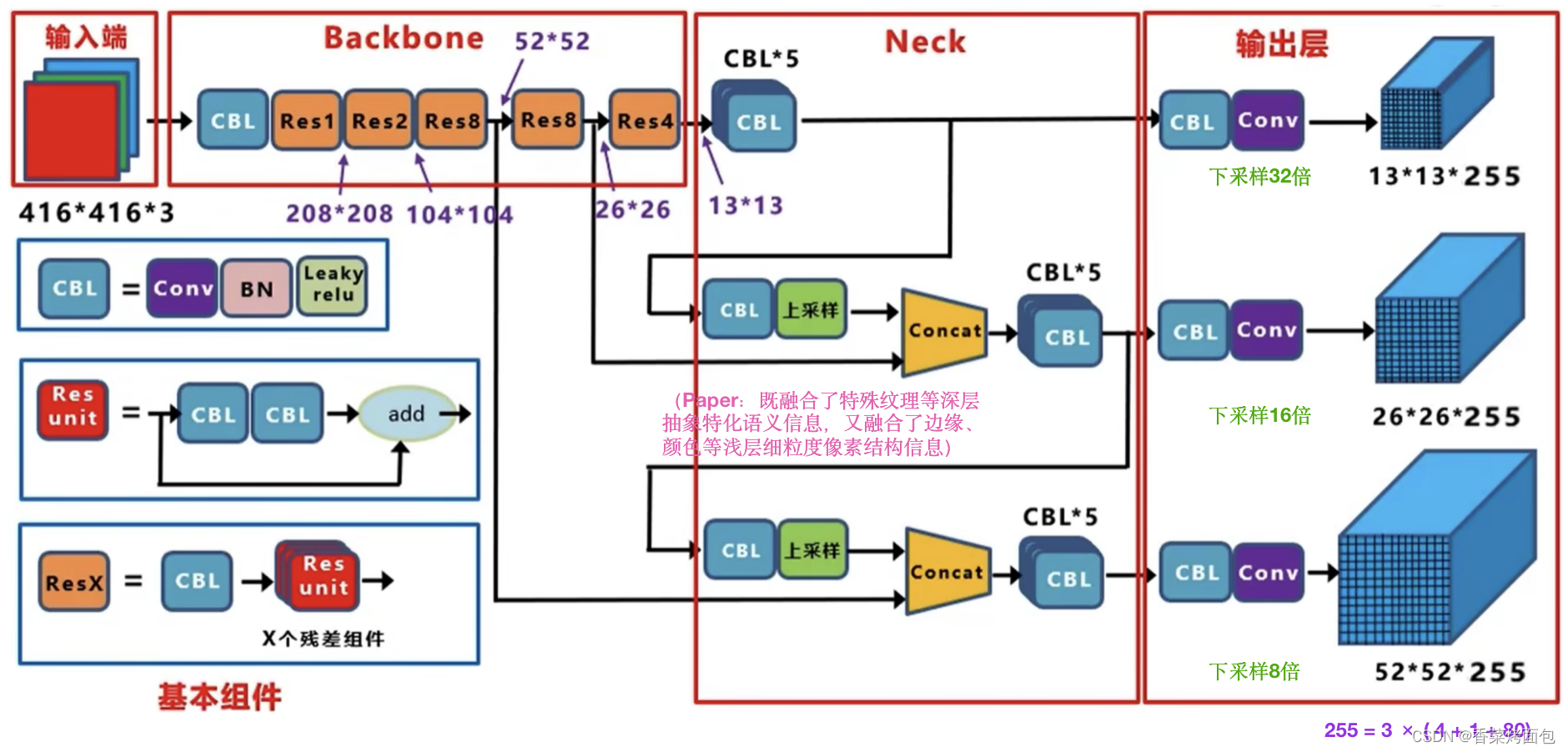
(Network structure diagram from Jiang Dabai)

Residual idea: Backbone DarkNet-53 draws on the residual idea of ResNet and uses a large number of residual connections in the basic network, so the network structure can be designed very deep, and the problem of gradient disappearance in training is alleviated, making the model easier convergence
Multi-layer feature map: Through upsampling and Concat operation, deep and shallow features are integrated, and finally output feature maps of 3 sizes, which is beneficial to multi-scale object and small object detection
No pooling layer: DarkNet-53 does not use pooling, and achieves the size reduction effect through a convolution kernel with a step size of 2, downsampling 5 times, and the overall downsampling rate is 32 (the input image size is a multiple of 32. , the larger the input, the larger the three feature maps obtained)

7.2 Backbone：Darknet-53

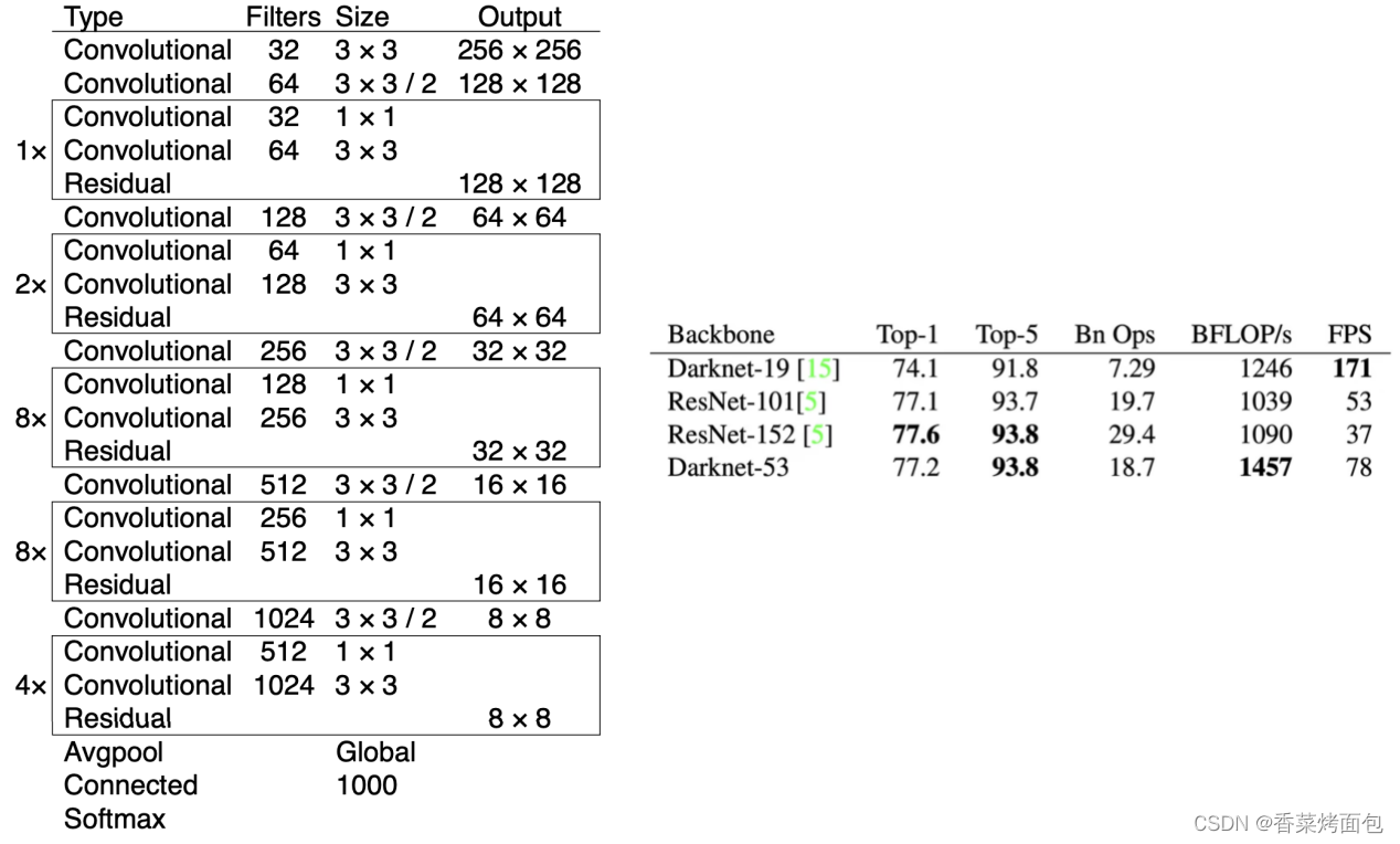
Backbone: DarkNet-53 (mixed DarkNet-19 and ResNet) - feature extractor (backbone network provides ingredients, followed by cooking, good ingredients may not make good meals, but without good ingredients, you can't cook good meals, backbone network extracted features)
Darknet-53 uses continuous 3 x 3 convolution and 1 x 1 convolution . There are a total of 53 weighted layers (52 convolutional layers + a full connection). For ResNet-152 and ResNet101, the classification accuracy is similar. Faster calculations and fewer network layers
Darknet-53 can use GPU more efficiently and perform forward inference faster (too many layers of ResNet)

YOLOv3 performed well at AP0.5, indicating that when the IOU threshold (which affects the division of positive and negative samples, thus affecting the model training results ) is set relatively small, the positioning may be correct; when the IOU threshold is increased, for example, to 0.95, the prediction box must be consistent with The GT is very coincident to determine that this frame is TP, and the prediction is correct. At this time, the performance of YOLOv3 is poor— the performance of precise positioning is poor
Improvements of YOLOv3 in small and dense targets :
- The number of grid cells is increased (YOLOv2 and YOLOv3 are compatible with any image size input - full convolutional network)
- Anchor for small targets is set
- Integrating multi-scale features for multi-scale prediction (FPN)
- The loss function adds a penalty small box term
- The network structure uses cross-layer connections and the feature extraction capability of the backbone network is enhanced

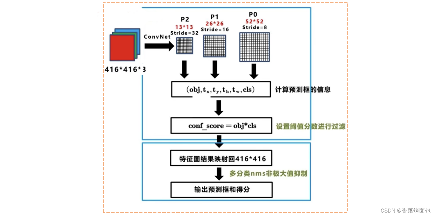
7.3 Mapping relationship between input and output

Input: 416x416 image, through the Darknet network to get prediction results of three different scales (inspired by the FPN feature pyramid), each scale corresponds to 255 channels (85 x 3), containing the predicted information, each grid Prediction results for anchors of each size
YOLOv1 : Input 448 x 448 , divided into 7 x 7 grid, no Anchor , generate B bbox (B=2), generate 7 x 7 x 2 = 98 prediction boxes , number of categories C=20, output tensor dimension 7 x 7 x (5 x B + C)
YOLOv2 : Input 416 x 416 , each grid cell has five Anchors , each grid cell corresponds to the original image receptive field size is the same, the size of the target is treated equally (pass through), 13 x 13 x 5 = 845 prediction boxes are generated , and the output Tensor dimensions are 13 x 13 x 5 x ( 5 + 20 )
YOLOv3 : Input 416 x 416 , generate 13 x 13 (large target), 26 x 26 (medium target), 52 x 52 (small target) three scale feature maps, three Anchor for each scale, generate (13x13 + 26x26 + 52x52) x 3 = 10647 prediction frames , each prediction corresponds to 85 dimensions, which are 4 (coordinate value), 1 (confidence score), 80 (coco category number)

7.4 YOLOv3 Anchor

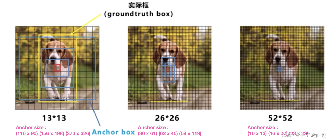
YOLOv3 assigns three Anchors (clustering) to each grid cell, a total of 9 Anchors
13 x 13 feature map : The receptive field corresponding to the original image is a grid cell corresponding to the 32 x 32 pixels of the original image, downsampled by 32 times, responsible for predicting large targets, corresponding to large Anchor
26 x 26 feature map : responsible for predicting the target
52 x 52 feature map : Responsible for predicting small targets

For example, for a target falling in a grid cell, the target is predicted by the Anchor with the largest IOU of the target ground truth in the Anchor of the grid cell, but each scale has an Anchor with the largest IOU, which scale grid cell What about the corresponding Anchor prediction?
The Anchor with the largest IOU of the target ground truth among all Anchors is responsible for predicting . YOLOv3 no longer looks at which grid cell the center point falls in, but who has the largest IOU

7.5 Positive and negative sample matching rules

Positive example: Take any ground truth, and calculate IOU with all 4032 boxes, and the predicted box with the largest IOU is a positive example
- A prediction frame can only be assigned to one ground truth responsible for prediction (the largest IOU)
- The positive example generates confidence loss, detection frame loss, and category loss. The corresponding category of the category label is 1, and the rest are 0, and the confidence label is 1.
Ignore the sample: except for the positive example, if the IOU with any ground truth is greater than the threshold (0.5 is used in the paper), it is an ignored sample
- Ignoring the sample does not generate any loss
Negative example: Except for the positive example (the detection frame with the largest IOU after the calculation of the ground truth, but the IOU is less than the threshold, it is still a positive example), and the IOU with all the ground truth is less than the threshold (0.5), then it is a negative example
- Negative examples only have confidence to generate loss, and the confidence label is 0

Note ⚠️:

YOLOv1 assigns the corresponding prediction box according to the center point, and YOLOv3 finds the prediction box with the largest IOU as a positive example according to the predicted value. This is because Yolov3 uses multi-scale feature maps , and there will be overlapping detection parts between feature maps of different scales , ignoring the samples It is the finishing touch in Yolov3
The confidence label in Yolov1/2 is the IOU between the predicted frame and the real frame , while Yolov3 is 0 and 1 , which means that the predicted frame is or is not a real object, which is a two-category
What's wrong with using IOU as a confidence threshold in Yolov1/2 ?
1. The highest IOU between many prediction boxes and gt is only 0.7 (this value is not high at all, it is difficult to train if this value is used as a label, if you directly set the label to 1, clearly tell the model that this is a positive sample, study hard, and learn as an idol , instead of just learning 0.7)
2. There are a lot of small objects in the COCO dataset, and the IOU is very sensitive to pixel offset and cannot be effectively learned——《Augmentation for small object detection》

7.5 Mapping relationship between input and output

7.6 Loss function

The following figure is from the analysis of the loss function of Tongji Zihao:

Note ⚠️: YOLOv3 tried to use Focal Loss , but the mAP was reduced by two points

Cause analysis: Focal Loss solves the problem of "unbalanced positive and negative samples and few really useful negative samples" in single-stage target detection, which is equivalent to a certain degree of difficult case mining. The IOU threshold of negative samples in YOLOv3 is set too high (0.5), which leads to the mixing of suspected positive samples (label noise) in negative samples, and Focal Loss will give these noises greater weight, so the effect is not good

7.7 Training process and testing process

7.8 Advantages and disadvantages of YOLOv3

Advantages of YOLOv3:

Fast inference speed and high cost performance
Low background false detection rate
Versatile

YOLOv3 disadvantages:

low recall
Poor positioning accuracy
Relatively weak detection ability for close or occluded groups and small objects