Table of contents
1.2 Absolute (value) loss function (absolute loss function)
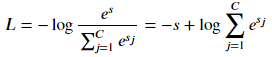
1.3 Logarithmic loss function (logarithmic loss function)
1.5 Image Comparison - Advantages and Disadvantages
2. Classification loss function
2.1 0-1 loss function (0-1 loss function)
2.2 Logarithmic likelihood loss function (Logistic loss)
2.3 Hinge loss function (Hinge loss)
2.4 Exponential loss function (Exponential loss)
2.5 Modified Huber loss function (Modified Huber loss)
2.6 Softmax loss (Softmax loss)
2.7 Image Comparison - Advantages and Disadvantages
3.4 Understanding regularization from multiple perspectives
1. Definition
Loss function (Loss Function) : It is defined on a single sample , refers to the error of a sample, and measures the quality of a prediction of the model .
Cost Function (Cost Function) = Cost Function = Experience Risk : It is defined on the entire training set, and is the average of all sample errors , that is, the average of all loss function values , and measures the quality of the model prediction in the average sense.
Objective function (Object Function) = structural risk = empirical risk + regularization term = cost function + regularization term : refers to the function that needs to be optimized in the end, and generally refers to structural risk. Regularizer = penalty term.
2. Loss function
1. Regression loss function
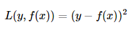
1.1 quadratic loss function
It is the single sample loss of MSE, also known as squared loss (squared loss), which refers to the square of the difference between the predicted value and the actual value. Sometimes for the convenience of derivation, a 1/2 is multiplied in front.
1.2 Absolute (value) loss function (absolute loss function)
It is MAE single sample loss, also known as absolute deviation (absolute Loss). The meaning of this loss function is similar to the above, except that the absolute value is taken instead of the sum of squares, and the gap will not be magnified by the square.

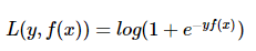
1.3 Logarithmic loss function (logarithmic loss function)
Also known as the log likelihood loss function (loglikelihood loss function), this loss function is more difficult to understand. In fact, the loss function uses the idea of maximum likelihood estimation.
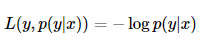
The popular explanation of P(Y|X) is: based on the current model, for sample X, its predicted value is Y, which is the probability of correct prediction. It can be obtained from the probability multiplication formula that the probabilities can be multiplied. In order to convert it into an addition, we take the logarithm. Finally, because it is a loss function, the higher the probability of correct prediction, the smaller the loss value should be, so add a negative sign to get an inversion.
Here are two points:
The first point is that the logarithmic loss function is very often used. Logistic regression, softmax regression, etc. all use this loss.
The second point is the understanding of this formula. This formula means that when the sample x is classified as y, we need to maximize the probability p(y|x). It is to use the currently known sample distribution to find the parameter value that is most likely to cause this distribution.
1.4 Huber loss (huber loss)

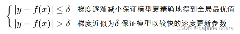
Where y is the real value, f(x) is the predicted value, and δ is the parameter of Huber Loss. When the predicted deviation is less than δ, it uses the square error, and when the predicted deviation is greater than δ, it uses the linear error. Compared with the linear regression of least squares, Huber Loss reduces the degree of punishment for outliers and is a commonly used robust regression loss function.
We noticed that a hyperparameter δ has been added to Huber Loss

The parameter δ plays a certain role in it, that is, when the prediction deviation is less than δ, the square error is used, which is what we call MSE, and when the prediction deviation is greater than δ, the linear error (similar to MAE) is used
In general, the optimal value of δ can be obtained through cross-validation
It can be seen that Huber Loss is a loss function with parameters used to solve regression problems in the application
1.5 Image Comparison - Advantages and Disadvantages
The most commonly used one is MSE square loss , but its disadvantage is that it will impose a large penalty on outliers, so it is not robust enough. If there are more abnormal points, the MAE absolute value loss performs better, but the disadvantage of the absolute value loss is that it is not continuous at y−f(x)=0y−f(x)=0, so it is not easy to optimize. Huber loss is a combination of the two. When |y−f(x)||y−f(x)| is less than a pre-specified value δ, it becomes a square loss, and when it is greater than δ, it becomes similar to absolute Value loss, so it is also a relatively robust loss function.
The graphic comparison of the three is as follows:

advantage
Enhanced outlier robustness of MSE reduces sensitivity to outliers
Using MAE when the error is large can reduce the influence of outliers and make the training more robust
The falling speed of Huber Loss is between MAE and MSE, which makes up for the slow falling speed of MAE in Loss and is closer to MSE
shortcoming
Additional hyperparameters δ
Reference: Huber loss of loss function Loss Function - Zhihu (zhihu.com)
2. Classification loss function
2.1 0-1 loss function (0-1 loss function)
That is, when the prediction is wrong, the loss function is 1, and when the prediction is correct, the loss function value is 0. This loss function does not consider the degree of deviation between the predicted value and the true value. As long as it is wrong, it is 1.
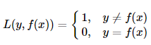

The 0-1 loss is discontinuous, non-convex, and non-leadable, and it is difficult to use the gradient optimization algorithm, so it is rarely used in daily life.
2.2 Logarithmic likelihood loss function (Logistic loss)
Logistic Loss is the loss function used in Logistic Regression.
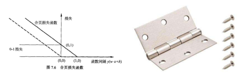
2.3 Hinge loss function (Hinge loss)
Hinge loss is usually used as a loss function in the SVM classification algorithm.


Hinge loss is the loss function used in svm, so that the sample loss of yf(x)>1 is all 0, which brings a sparse solution, so that svm can determine the final hyperplane with only a few support vectors .
In addition, the following form is also the formula expression of Hinge loss:

The first term is the loss and the second term is the regularization term. This formula means that when yi(w·xi+b) is greater than 1, the loss is 0, otherwise the loss is 1−yi(w·xi+b). Compared with the loss function [−yi(w·xi+b)] of the perceptron, Hinge loss must not only be classified correctly, but also when the confidence level is high enough, the loss will be 0, which has higher requirements for learning. Comparing the images of perceptron loss and Hinge loss, it is obvious that Hinge loss is more stringent.
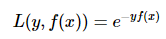
2.4 Exponential loss function (Exponential loss)
Exponential Loss is generally used in AdaBoost . Because using Exponential Loss, it is more convenient to use the additive model to derive the AdaBoost algorithm. This loss function is more sensitive to outliers and less robust than other loss functions.

2.5 Modified Huber loss function (Modified Huber loss)
Huber Loss integrates the advantages of MAE and MSE, and with a slight improvement, it can also be used for classification problems, called Modified Huber Loss.
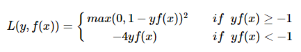

The modified huber loss combines the advantages of hinge loss and logistic loss. It can not only generate sparse solutions when yf(x)>1 to improve training efficiency, but also perform probability estimation. In addition, its penalty for (yf(x)<−1) samples increases linearly, which means that it is less disturbed by outliers and has better robustness. The SGDClassifier in scikit-learn also implements modified huber loss.
2.6 Softmax loss (Softmax loss)
The Softmax layer of the machine learning model, the output of the correct class pair is:
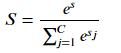
Among them, C is the number of categories, the lowercase letter s is the Softmax input corresponding to the correct category, and the uppercase letter S is the Softmax output corresponding to the correct category.

In the figure above, when s << 0, Softmax is approximately linear; when s>>0, Softmax tends to zero. Softmax is also less disturbed by outliers and is mostly used in neural network multi-classification problems.
2.7 Image Comparison - Advantages and Disadvantages

It is worth noting that the direction of the modified huber loss in the above figure is similar to the exponential loss, and its robust properties cannot be seen. In fact, this is the same as the time complexity of the algorithm, and the huge difference can only be reflected after being multiplied:

3. Regularization
3.1 Definition
Here we first need to understand the principle of structural risk minimization :
On the basis of empirical risk minimization (training error minimization), use as simple a model as possible to improve the prediction accuracy of model generalization
Our so-called regularization is to add some regularization items, or model complexity penalty items (to prevent model overfitting) on the basis of the original Loss Function. Take our linear regression as an example.
3.2 L1 and L2 regularization
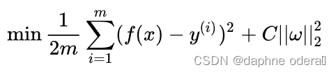
Optimization objective (loss function):

Add L1 regular term (lasso regression):

Add the L2 regular term (Ridge regression):
Next, we need to understand how the final solution changes when the objective function is solved after adding the regularization term. Let's understand it from an image perspective:
Assuming that X is a two-dimensional sample, the parameters to be solved are also two-dimensional. The figure below is called the contour plot of the original function curve. For each group of contour lines (same color) of the objective function in the figure, the input values are all the same, which represents multiple groups of solutions.
Contour Function Diagram of Primitive Function

Function image after adding L1 and L2 regular terms
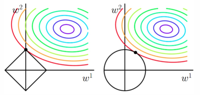
Comparing the two pictures we can see that:
-
If the L1 and L2 regularization terms are not added, for a convex function such as the linear regression loss function, our final result is the point on the contour line of the innermost purple circle.
-
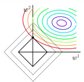
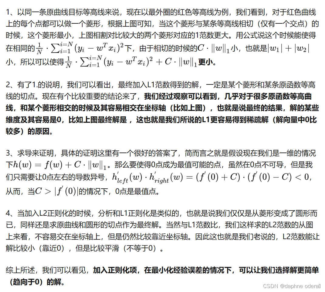
When adding L1 regularization, we first draw the image of |w1|+|w2|=F, which is this rhombus. At this time, our goal is not only to make the original curve value smaller (closer to the center purple circle), but also to make the rhombus as small as possible (the smaller the F, the better). Then if it is the same as the original solution, the rhombus is obviously very large.
L1 norm solution diagram
3.3 Solving
3.4 Understanding regularization from multiple perspectives
For details, please see: A more comprehensive explanation of L1 and L2 regularization (qq.com)
The difference between L1 regularization and L2 regularization:
L1 regularization is to add the L1 norm after the loss function, so that it is easier to find a sparse solution. L2 regularization is to add the L2 norm (square) after the loss function. Compared with the L1 regularization, the obtained solution is smoother (not sparse), but it can also guarantee the comparison of dimensions close to 0 (not equal to 0) in the solution. more, reducing the complexity of the model.
Loss function part reference:
https://zhuanlan.zhihu.com/p/358103958
https://www.zhihu.com/question/47746939
https://blog.csdn.net/dream_to_dream/article/details/117745828
http://www.javashuo.com/article/p-fohpuvmc-ms.html
Regularization part content reference: