Article directory
Reference link: https://blog.csdn.net/v_JULY_v/article/details/81410574
foreword
Ensemble learning : complete learning tasks by constructing and combining multiple learners, that is, first generate a group of individual learners, and then combine them with a certain strategy. Individual learners are derived from an existing learning algorithm Generated from the training data, at the same time, it must have a certain accuracy, not be too bad, have diversity, and have differences between learners. The ensemble learner significantly increases the generalization performance.
However, diversity and accuracy are contradictory. When accuracy increases, diversity will be sacrificed. How to generate good and different learners is the focus of integrated learning.
Two branches: Boosting and Bagging, the former generates serialization serially through strong dependencies between individual learners; the latter generates parallel methods without strong dependencies between individual learners.
1. Boosting
A set of methods to promote a weak learner to a strong learner: increase the weight of misclassified samples and reduce the weight of correctly classified samples, so that the algorithm pays more attention to misclassified samples.
Working mechanism:
First, a weak learner 1 is trained from the training set with the initial weight, and the weight of the training samples is updated according to the performance of the learning error rate of the weak learning, so that the weight of the training sample points with a high learning error rate of the previous weak learner 1 is becomes higher, so that these points with high error rates get more attention in the following weak learner 2. Then the weak learner 2 is trained based on the weight-adjusted training set, and this is repeated until the number of weak learners reaches the number T specified in advance, and finally these T weak learners are integrated through the ensemble strategy to obtain the final strong learner.
(1)Adaboost
AdaBoost is a classic algorithm in Boosting, which is mainly used in binary classification problems.
The Adaboost algorithm adjusts the sample distribution by adjusting the sample weight, that is, increasing the weight of the samples misclassified by the previous round of individual learners, and reducing the weight of those correctly classified samples , so that the misclassified samples can be affected by More attention, so that it can be correctly classified in the next round, makes the classification problem "divide and conquer" by a series of weak classifiers. For the combination method, AdaBoost adopts the method of weighted majority voting. The additive model means that the strong classifier is linearly added by a series of weak classifiers. Specifically, increase the weight of the Ruo classifier with a small classification error rate, and decrease the weight of the Ruo classifier with a large classification error rate, so as to adjust their role in voting. The AdaBoost algorithm is a binary classification algorithm when the model is an additive model, the loss function is an exponential function, and the learning algorithm is a forward step-by-step algorithm.
(2) GBDT (Gradient Boosting Decision Tree) Gradient Boosting Tree
GBDT is the accumulation of the output prediction values of multiple trees, and the trees of GBDT are all regression trees rather than classification trees.
The gradient boosting tree is to solve the optimization algorithm of the boosting tree when the loss function is a general loss function. It is called the gradient boosting algorithm. It uses the approximation method of the steepest descent method. The key is to use the negative gradient of the loss function in the value of the current model.
The specific method is to initialize the loss parameter first, then calculate the loss function, and derive its derivative value to fit a regression tree to obtain the node area. Use the negative gradient of the loss function as the residual (second-order Taylor expansion),
Two, bagging and random forest
(1) Bagging
The algorithm principle of Bagging is different from that of boosting. Its weak learners have no dependencies and can be generated in parallel.
Working Mechanism:
The training set of individual weak learners of bagging is obtained by random sampling. Through T times of random sampling, we can obtain T sampling sets. For these T sampling sets, we can independently train T weak learners, and then use the set strategy to obtain the final T weak learners. strong learner.
The bootstap sampling method is generally used here, that is, for the original training set of m samples, we randomly collect a sample each time and put it into the sampling set, and then put the sample back, that is to say, when sampling next time The sample is still likely to be collected, so that m times are collected, and finally a sampling set of m samples can be obtained. Since it is a random sampling, each sampling set is different from the original training set, and is also different from other sampling sets. , so that multiple different weak learners are obtained.
The complexity of training a Bagging ensemble is the same as directly using the base classifier algorithm to train a learner, indicating that Bagging is an efficient ensemble learning algorithm.
(2) Random Forest (RF for short)
Random forest is an extension of bagging. On the basis of constructing Bagging ensemble with decision tree as the base learner , RF further introduces random attribute selection in the training process of decision tree . In the process of generating individual learners, not only sample disturbance but also attribute disturbance are added. Specifically, the traditional decision tree selects an optimal attribute in the attribute set of the current node (assuming that there are d attributes) when selecting the partition attribute, while in RF, for each node of the base decision tree, start with From the attribute set of the node, k attributes are randomly selected to form the attribute set, and then the optimal partition attribute is selected from the attribute set. In general, k=log2d is recommended.
Advantages of random forests:
1. It can handle very high-dimensional data without feature selection;
2. After the training is completed, which attributes are more important can be given;
3. It is easy to make a parallel method and the speed is fast;
4. It can be visualized and displayed. Easy to analyze.
Comparison of Random Forest and Bagging:
1. The convergence of the two is similar, but the initial performance of RF is relatively poor, especially when there is only one base learner. Random forests generally converge to lower generalization error as the number of base learners increases.
2. The training efficiency of random forest is often better than that of Bagging, because Bagging is a "deterministic" decision tree, while random forest uses a "random" decision tree.
3. XGBoost
XGBoost (eXtreme Gradient Boosting), a scalable machine learning system for tree boosting, is integrated by many CART trees. This system can be used as an open source software package. The excellent version of GBDT belongs to the boosting method.
CART tree (Classification And Regression Tree, collectively referred to as classification tree and regression tree) CART uses the Gini index, the smaller the Gini index, the higher the purity of the data set; 1.
Classification tree : the sample output (ie, the response value) is in the form of a class, For example, judging whether the medicine is real or fake, whether to go to the movies on weekends or not. The goal of classification is to judge which known sample class a new sample belongs to based on certain characteristics of known samples, and its result is a discrete value.
ID3 information gain: 
Gain rate for C4.5
2. The sample output of the regression tree is in the form of a value. For example, the amount of a housing loan issued to someone is a specific value, which predicts the probability of cancer. The results of the regression are continuous values. The regression tree assumes that the tree is a binary tree, and continuously splits the features. For example, the current tree node is split based on the jth eigenvalue. If the eigenvalue is less than s, the sample is divided into the left subtree, and the sample greater than s is divided into the right subtree. The essence is to divide the sample space in this feature dimension divided.
Objective function: 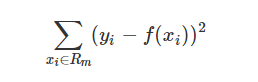
When we want to solve the optimal segmentation feature j and the optimal segmentation point s, it is transformed into solving such an objective function: 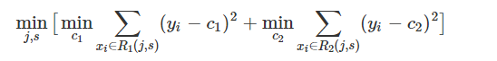
as long as all the segmentation points of all features are traversed, the optimal segmentation point can be found features and segmentation points. Finally, a regression tree is obtained.
Derivation of the objective function:
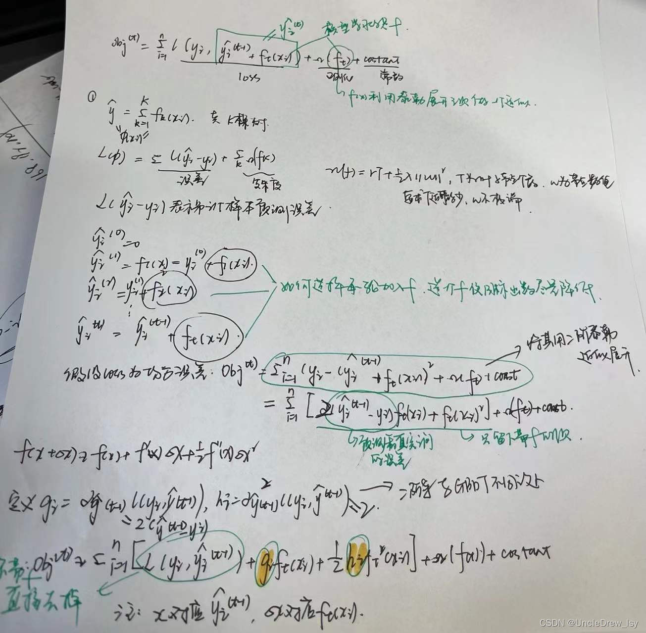
Bring in the regularization term:
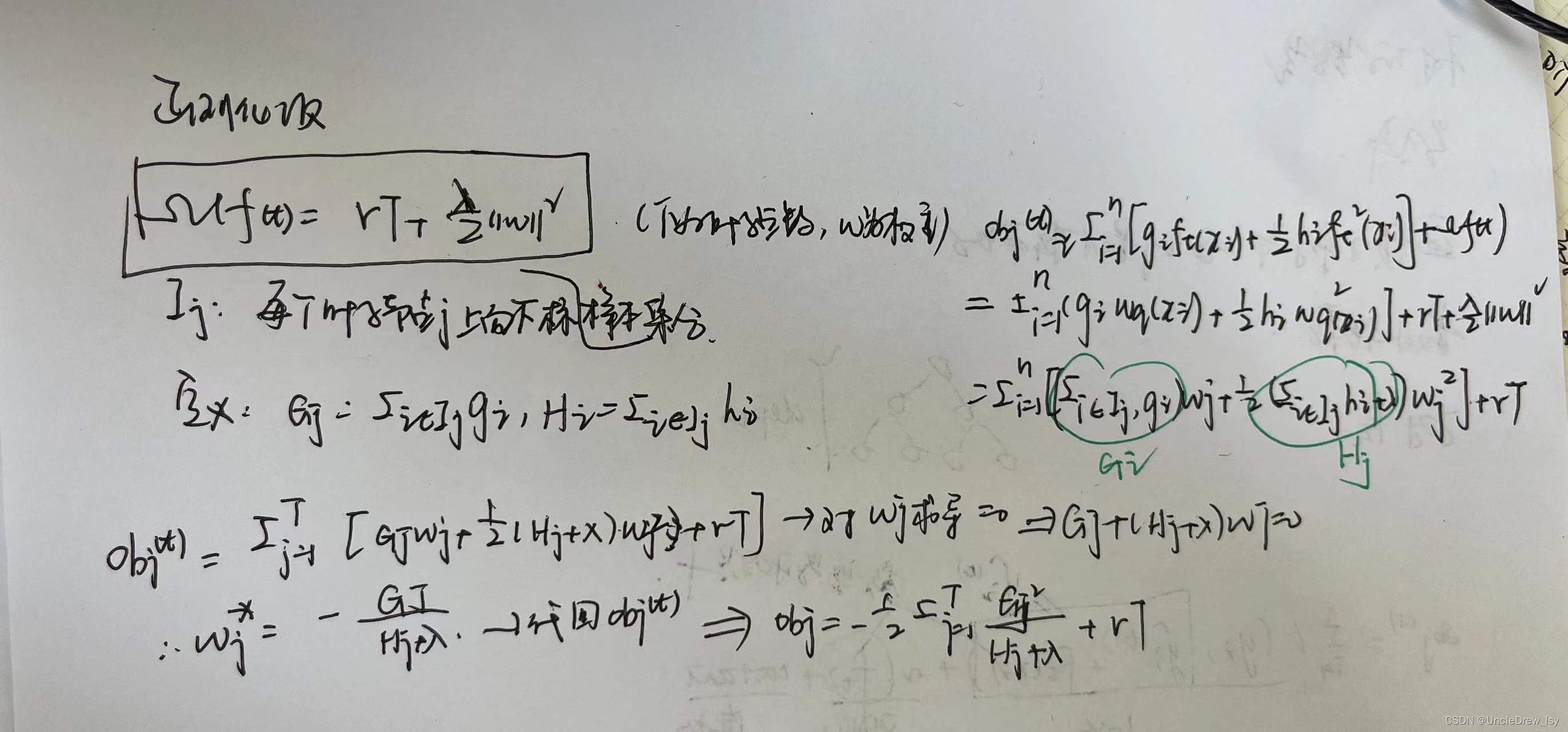
3. How the tree is constructed:
1) Greedy method to enumerate all different tree structures
The current situation is that as long as the tree structure is known, the best score under the structure can be obtained, so how to determine the tree structure?
One way to take it for granted is: constantly enumerate the structures of different trees, and then use the scoring function to find a tree with an optimal structure, then add it to the model, and repeat this operation. And if you think about it again, you will realize that there are too many states to enumerate, which are basically infinite, so what should you do?
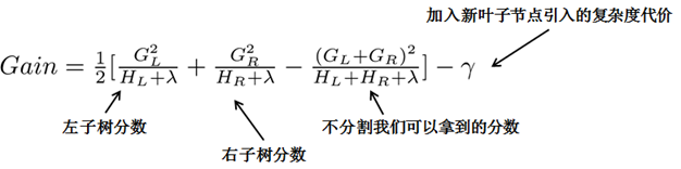
Let's try the greedy method. Starting from tree depth 0, each node traverses all features, such as age, gender, etc., and then for a feature, first sort according to the value in the feature, and then linearly scan the feature and then Determine the best segmentation point, and finally divide all the features, we choose the feature with the highest so-called gain Gain, and how to calculate Gain?
(2) Approximate algorithm
is mainly for data too large to be calculated directly.
When the gain brought by the introduced split is less than the set threshold, we can ignore this split, so not every split will increase the overall loss function, which is a bit of pre-pruning. The threshold parameter is (that is, the regular term The coefficient of the number of leaf nodes T in the tree);
when the tree reaches the maximum depth, stop building the decision tree, and set a hyperparameter max_depth to avoid too deep a tree and cause local samples to be learned, thereby overfitting;
when the sample weight sum is less than the set threshold then stop building. What does it mean, that is, it involves a hyperparameter - the minimum sample weight and min_child_weight, which are similar to GBM's min_child_leaf parameter, but not exactly the same. The general idea is that there are too few samples of a leaf node, and the termination is also to prevent overfitting;
Original link: https://blog.csdn.net/v_JULY_v/article/details/81410574