The core of the GBDT algorithm is: first construct a (decision) tree, and then continuously construct a tree on the residuals of the existing model and the actual sample output , and iterate in turn.
table of Contents
Decistion Tree (decision tree)
Multi-classification algorithm
Two different versions of GBDT
Advantages and disadvantages of GBDT algorithm
GBDT is also a member of the integrated learning Boosting family, but it is very different from the traditional Adaboost.
Looking back at AdaBoost ( integrated learning-Boosting integrated learning algorithm AdaBoost ), we use the error rate of the previous iteration of the weak learner to update the weights of the training set samples, and this round of iteration continues.
GBDT is iterative, it is a decision tree based on the accumulated iterative algorithm, which is configured by a set of weak learner (tree), and the results added up multiple satellites decision tree output as the final prediction, the weak learner defines only Use CART regression tree model. The GBDT algorithm has many names, but they are all the same algorithm:
GBRT (Gradient Boost Regression Tree) progressive gradient regression tree
GBDT (Gradient Boost Decision Tree) progressive gradient decision tree
MART (MultipleAdditive Regression Tree) multi-decision regression tree
The GBDT algorithm is mainly composed of three parts:
Decistion Tree (ie DT regression tree)
Gradient Boosting (ie GB gradient boost)
Shrinkag (gradient)
Decistion Tree (decision tree)
When mentioning decision trees (DT, Decision Tree), the first thing most people think of is the C4.5 classification decision tree. But if you think of the tree in GBDT as a classification tree from the beginning, it is a wrong understanding, so don't think that GBDT is a lot of classification trees.
Decision trees are divided into two categories, regression trees and classification trees. The former is used to predict real values, such as tomorrow’s temperature, the user’s age, and the degree of relevance of the webpage; the latter is used to classify label values, such as sunny/cloudy/fog/rain, user gender, and whether the webpage is spam. What I want to emphasize here is that the addition and subtraction of the results of the former is meaningful, such as 10 years old + 5 years-3 years = 12 years old, the latter is meaningless, such as male + male + female = male or female? The core of GBDT is to accumulate the results of all trees as the final result , just like the previous accumulation of age (-3 is plus minus 3), and the results of the classification tree obviously cannot be accumulated, so the trees in GBDT are all regressions. The tree is not a classification tree. This is very important for understanding GBDT (although GBDT can also be used for classification after adjustment, it does not mean that GBDT's tree is a classification tree).
Classification tree
Each time the classification tree is branched, each feature value of each feature is exhausted, and the feature splitting method that maximizes the entropy is found, and two new nodes are obtained by branching according to the standard, and the same method is used to continue branching until everyone All are classified into leaf nodes with unique gender, or reach a preset termination condition. If the category in the final leaf node is not unique, the category of the majority is used as the category of the leaf node.
Regression tree
The overall process of the regression tree is similar, but each node (not necessarily a leaf node) will get a predicted value. Taking age as an example, the predicted value is equal to the average age of all people belonging to this node. When branching, exhaust each threshold of each feature to find the best segmentation point, but the best measure is no longer the maximum entropy, but to minimize the mean square error , such as (each person's age-predicted age) ^2 The sum of / N, or the sum of squared prediction errors for each person divided by N. This is easy to understand. The more people who are predicted to make mistakes, the more outrageous they are, and the larger the mean square error. The most reliable branching basis can be found by minimizing the mean square error. Branch until the age of the person on each leaf node is unique (this is too difficult) or reach a preset termination condition (such as the upper limit of the number of leaves), if the age of the person on the final leaf node is not unique, the The average age of everyone is used as the predicted age of the leaf node.
The basic process of classification tree and regression tree is consistent with finding the threshold (split value) according to the feature, but the measurement standard of the threshold is different, that is, the selected optimization function is different. The criterion for selecting the threshold of the classification tree is to realize that each branch has only one classification as much as possible, that is, in the gender classification, as many male branches as possible are males and as few females as possible; as many female branches as possible are females , As few men as possible. In mathematics, the ratio of men to women is 1:1. The criterion for selecting the threshold of the regression tree is to minimize the mean square error between the predicted value and the true value.
Regression and classification use different methods to achieve the goal of "dynamically determining sample weights". Regression uses fitting residuals, and classification uses error rates to adjust sample weights.
Gradient Boosting
The method of improvement is based on the idea that for a complex task, the judgement obtained by appropriately synthesizing the judgements of multiple experts is better than the judgement of any one of the experts alone. This view of gradient boosting in the function domain has a profound impact on many areas of machine learning.
Boosting is a machine learning technique that can be used for regression and classification problems. It generates a weak prediction model (such as a decision tree) at each step, and weights it to the total model, and finally brings a strong prediction model; if each step is weak The prediction model generation is based on the gradient direction of the loss function , which is called gradient boosting.
The gradient lifting algorithm first gives a target loss function whose domain is a set of all feasible weak functions (basis functions); the lifting algorithm gradually approaches the local minimum by iteratively selecting a basis function in the direction of the negative gradient .
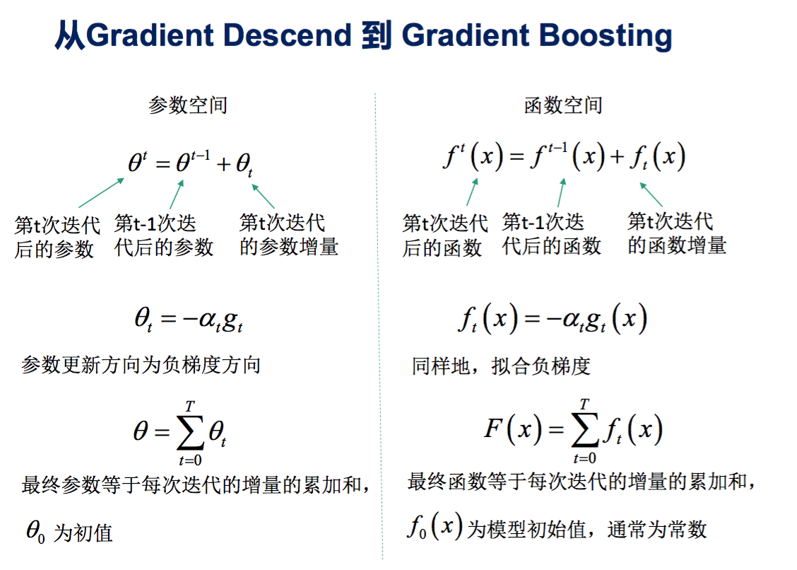
The gradient boosting algorithm is actually the same as the gradient descent algorithm, but the angle of the problem is different . For example, in linear regression, we use gradient descent to optimize the parameters so that the loss function can reach the (local) minimum; if we change the angle , What we optimize is not the parameter, but this function, and then through the method of descending along the gradient direction to reach the (local) minimum of the loss function, it becomes the gradient boosting algorithm.
The following figure shows the comparison of gradient boosting algorithm and gradient descent algorithm. It can be found that both of them use the information of the negative gradient direction of the loss function relative to the model to update the current model in each iteration, but in the gradient descent, the model is expressed in parameterized form, so that the model The update is equivalent to the parameter update. In gradient boosting, the model does not need to be parameterized, but is directly defined in the function space, which greatly expands the types of models that can be used.

The original Boost algorithm (such as Adaboost) assigns a weight value to each sample at the beginning of the algorithm. At the beginning, everyone is equally important. The model obtained in each step of training will make the estimation of the data point correct or wrong. After each step, we increase the weight of the wrong point and reduce the weight of the paired point, so that some points If you are always classified as wrong, you will be "seriously concerned" and will be given a high weight. Then wait for N iterations (specified by the user), and N simple classifiers (basic learners) will be obtained, and then we will combine them (for example, we can weight them, or let them vote, etc.), Get a final model.
Each tree of GBDT learns the residuals of the conclusion sums of all previous trees. This residual is a cumulative amount that can get the true value after adding the predicted value. For example, the true age of A is 18 years old, but the predicted age of the first tree is 12 years old, and the difference is 6 years, that is, the residual is 6 years old. Then in the second tree we set the age of A to 6 years old to study. If the second tree can really divide A into 6-year-old leaf nodes, the result of adding up the two trees is A's true age. If the conclusion of the second tree is 5 years old, then A still has a residual error of 1 year, and the age of A in the third tree becomes 1 year old. Continue to learn, this is the meaning of Gradient Boosting in GBDT.
The difference between Gradient Boost and traditional Boost is that each calculation is to reduce the last residual (residual), and in order to eliminate the residual, we can establish a new gradient in the direction of the residual reduction (Gradient) model. Therefore, in Gradient Boost, each new model is created to reduce the residual of the previous model in the direction of the gradient, which is very different from traditional Boost for weighting correct and incorrect samples.
In linear regression, we hope to find a set of parameters to minimize the residuals of the model. If only the first term is used to explain the quadratic curve, then there will be a lot of residuals. At this time, the quadratic term can be used to continue to explain the residuals, so this quadratic term can be added to the model. Similarly, GB first calculates the pseudo-residuals according to the initial model, and then builds a learner to interpret the pseudo-residuals, which reduces the residuals in the gradient direction. Multiply the learner by the weight coefficient (learning rate) and linearly combine the original model to form a new model. In this way, iterative iterations can find a model that minimizes the expected loss function.
In general, for a sample, the ideal gradient is the gradient closer to 0. Therefore, we need to be able to make the estimated value of the function able to make the gradient move in the opposite direction (in the dimension >0, move in the negative direction, and in the dimension <0, move in the positive direction) and finally make the gradient as far as possible = 0), and the The algorithm will pay serious attention to those samples with relatively large gradients, which is similar to Boost. After getting the gradient, how to reduce the gradient. Here is an iteration + decision tree method. When initializing, give an estimated function F(x) (you can let F(x) be a random value, or you can let F(x)=0) , And then build a decision tree based on the current gradient of each sample at each iteration step. Let the function go in the opposite direction of the gradient, and finally make the gradient smaller after N iterations. The decision tree established here is not the same as the ordinary decision tree. First, this decision tree has a fixed number of leaf nodes J. After J nodes are generated, no new nodes are generated.
Shrinkage (gradient)
Shrinkage is the third basic concept of GBDT, which means "reduction" in Chinese. Its basic idea is that it is easier to avoid over-fitting than the way of quickly approximating the result by taking a small step each time. In other words, the reduction thought does not fully trust each residual tree. It believes that each tree has only learned a small part of the truth, and only a small part of the truth is accumulated when accumulating. Only by learning a few more trees can the deficiency be made up.
Shrinkage is not the step size of Gradient. Shrinkage is just a step-by-step refinement method that changes from large steps to small steps. This looks very similar to Gradient target = Gradient unit direction * step length. But it's actually very different:
(1) The processing object of shrinkage is not necessarily the Gradient direction, but also the residual, which can be any increment, that is, target=anything*shrinkage step size.
(2) Shrinkage determines the size of the final step, not the size of the desired step. The former is to discount the existing learning results, and the latter is responsible for how far to go in the local optimal direction when determining the learning goal.
(3) Setting a smaller shrinkage will only make learning slower. Setting a larger shrinkage means no setting. It is suitable for all incremental iterative solving problems; while setting the step size of Gradient is smaller, it is easy to fall into the local optimum. Does not converge. It is only used to solve with gradient descent. The two are actually not much related. LambdaMART actually uses both, and the externally configurable parameter is shrinkage instead of Gradient step size.
That is, Shrinkage still uses the residual as the learning target, but for the results of residual learning, only a small part (step*residual) is accumulated to gradually approach the target. The step is generally small, such as 0.01~0.001 (note that the step is not gradient The step), resulting in the residual error of each tree is gradual rather than abrupt. Intuitively, this is also very easy to understand. It's not like using the residual to fix the error in one step, but only a little bit. In fact, it cuts the big step into many small steps. Essentially, Shrinkage sets a weight for each tree , and this weight is multiplied when accumulating , but it has nothing to do with Gradient . This weight is step. Just like Adaboost, Shrinkage can reduce the occurrence of over-fitting is also empirically proved, and there is no theoretical proof yet.
GBDT algorithm flow
Regression algorithm
Input: number of training sample
iterations (number of base learners): T
loss function: L
output: strong learner H(x)

Two classification algorithm

Multi-classification algorithm

GBDT loss function

Here we look at the GBDT classification algorithm. The classification algorithm of GBDT is not different from the regression algorithm of GBDT in thought, but because the sample output is not a continuous value, but a discrete category, we cannot directly fit the category from the output category. The error of the output.
In order to solve this problem, there are two main methods. One is to use an exponential loss function. At this time, GBDT degenerates to the Adaboost algorithm. Another method is to use a method similar to the log-likelihood loss function of logistic regression. In other words, we use the difference between the predicted probability value of the category and the true probability value to fit the loss. This article only discusses the GBDT classification using the log-likelihood loss function.
GBDT regularization
For GBDT regularization, we use the sub-sampling ratio method and the defined step size v method to prevent over-fitting.
-
**Subsampling ratio:** The subsample ratio of sampling without replacement (subsample), the value is (0,1]. If the value is 1, then all samples are used. If the value is less than 1, the part is used Samples are used for GBDT decision tree fitting. Choosing a ratio of less than 1 can reduce variance and prevent overfitting, but it will increase the deviation of sample fitting. Therefore, the value should not be too low, and it is recommended to be between [0.5, 0.8].
-
**Define the step size v: **For the iteration of the weak learner, we define the step size v with a value of (0,1]. For the same training set learning effect, a smaller v means we need more The number of iterations of the weak learner. Usually we use the step size and the maximum number of iterations together to determine the fitting effect of the algorithm.
Two different versions of GBDT
There are currently two different description versions of GBDT, both of which have their own supporters. Pay attention to the distinction when reading the literature.
The residual version describes GBDT as a residual iteration tree, thinking that each regression tree is learning the residuals of the previous N-1 trees. This version is also used in the ELF open source software implementation.
The Gradient version describes GBDT as a gradient iteration tree and uses the gradient descent method to solve it. It is believed that each regression tree learns the gradient descent value of the previous N-1 trees. This version was introduced in the previous leftnoteasy blog, the source code of umass This version is used in the implementation (to be precise, the MART in LambdaMART is this version, and the MART implementation is the previous version).
In general, the two are the same in that they are both iterative regression trees, and both add up the results of each tree as the final result (Multiple Additive Regression Tree), and each tree has N-1 tree deficiencies before learning. There is no difference between the two in terms of overall process and input and output; the difference between the two is mainly whether to use Gradient as the solution method during each iteration. The former uses residual instead of Gradient. The residual is the global optimal value. Gradient is the local optimal direction * step size, that is, the former tries to make the result the best at every step, and the latter tries to make the result better at every step. better.
Both advantages and disadvantages. It seems that the former is a little more scientific, and there is an absolute optimal direction that is not learned. Why do you try to estimate a local optimal direction by looking for a distance? The reason is flexibility. The biggest problem with the former is that because it relies on residuals, the cost function is generally fixed to reflect the mean square error of the residuals, so it is difficult to deal with problems other than pure regression problems. The latter solution method is gradient descent, as long as the derivable cost function can be used, so LambdaMART for sorting is the latter.
Boost in GBDT is an iteration of sample targets, not an iteration of re-sampling, nor Adaboost.
Boosting in Adaboost refers to assigning different weights from the samples according to the right or wrong classification, and using these weights when calculating the cost function, so that "the weight of the wrongly divided samples becomes larger and larger until they are matched". Bootstrap also has a similar idea, but it can use different weights as sample probabilities to re-sample the training sample set, so that the wrongly classified samples are further learned, and the correctly classified samples do not need to be learned again. But the boost in GBDT is completely different and has nothing to do with the above logic. The sample set of each step of boost in GBDT is unchanged, and what changes is the regression target value of each sample.
sklearn parameters
GradientBoostingRegressor(loss=’ls’, learning_rate=0.1, n_estimators=100,
                subsample=1.0, criterion=’friedman_mse’, min_samples_split=2,
                min_samples_leaf=1, min_weight_fraction_leaf=0.0, max_depth=3,
                min_impurity_decrease=0.0, min_impurity_split=None, init=None,
                random_state=None, max_features=None, alpha=0.9, verbose=0,
                max_leaf_nodes=None, warm_start=False, presort=’auto’,
                validation_fraction=0.1, n_iter_no_change=None, tol=0.0001)
Parameter Description:
- n_estimators: The maximum number of iterations of weak learners, that is, the number of largest weak learners.
- learning_rate: step size, that is, the weight reduction coefficient a of each learner, which is one of the regularization methods of GBDT.
- subsample: sub-sampling, the value is (0,1]. Deciding whether to sample the original data set and the sampling ratio is also one of the GBDT regularization methods.
- init: Weak learner when we initialize. If not set, the default is used.
- loss: loss function, optional {'ls'-square loss function,'lad' absolute loss function-,'huber'-huber loss function,'quantile'-quantile loss function}, the default is'ls'.
- alpha: When we are using Huber loss "Huber" and quantile loss "quantile", we need to specify the corresponding value. The default value is 0.9. If there are more noise points, this quantile value can be appropriately reduced.
- criterion: The criterion for searching the optimal split point in the decision tree section. The default is "friedman_mse", and "mse"-mean square error and'mae"-absolute error are optional.
- max_features: The maximum number of features considered during division, which is the meaning of feature sampling, and all features are considered by default.
- max_depth: The maximum depth of the tree.
- min_samples_split: The minimum number of samples required for subdividing internal nodes.
- min_samples_leaf: The minimum number of samples of leaf nodes.
- max_leaf_nodes: Maximum number of leaf nodes.
- min_impurity_split: The minimum impurity of node division.
- presort: Whether to sort the data in advance to speed up the search for the optimal split point. The default is pre-sort. If it is sparse data, it will not be pre-sorted. In addition, sparse data cannot be set to True.
- validation fraction: The percentage of validation data reserved for early stopping. Only available when n_iter_no_change is set.
- n_iter_no_change: When the verification score does not improve, it is used to decide whether to use early stop to terminate the training.
Advantages and disadvantages of GBDT algorithm
Advantages of GBDT
(1) Prevent over-fitting;
(2) The residual calculation of each step actually increases the weight of the wrong instance in disguise, while the instance that has already been paired tends to 0;
(3) The residual is the absolute direction of the global optimum;
(4) Use some robust loss functions, which are very robust to outliers. Such as Huber loss function and Quantile loss function.
Disadvantages of GBDT
(1) Boost is a serial process , which is not easy to parallelize, and the calculation complexity is high , which is relatively time-consuming (large data volume is very time-consuming);
(2) At the same time, it is not suitable for high-dimensional features. If the data dimension is high, the calculation complexity of the algorithm will be increased. For the specific complexity, please refer to the improvement points of XGBoost and lightGBM;
Reference link: https://zhuanlan.zhihu.com/p/58105824
Reference link: https://www.jianshu.com/p/b954476a00d9
Reference link: https://www.zybuluo.com/Dounm/note/1031900
Reference link: https://zhuanlan.zhihu.com/p/30736738
Reference link: https://blog.csdn.net/XiaoYi_Eric/article/details/80167968