1. What is the difference between pytorch and tensorflow?
1. The first is the creation and debugging
of the graph. The creation of the pytorch graph structure is dynamic, that is, the graph is created at runtime, and it is easier to debug the pytorch code. The
creation of the tensorflow graph structure is static, that is, the graph is first "compiled", and then run.
(A good framework should have three points:
——It is convenient to realize large calculation graph;
——It can automatically find the derivative of variables;
——It can be easily run on GPU;
pytorch has done it, but now many companies use it. It is TensorFlow, and pytorch is used more in academic research because of its flexibility. I think it is possible. Google may start earlier, and Facebook is a latecomer. Although it is flexible, many companies have already entered the pit of TensorFlow. It still takes a lot of effort to migrate all of them; moreover, TensorFlow is better at GPU distributed computing, and its efficiency is higher than that of pytorch when the amount of data is huge . I think this is also an important reason.)
2. In terms of flexibility,
pytorch is a dynamic calculation graph. Data parameters can be migrated between CPU and GPU very flexibly. It is easy to debug.
Tensorflow is a static calculation graph. It is troublesome to migrate data parameters between CPU and GPU, and debugging is troublesome.
3. Device management - (memory, video memory)
tensorflow : No manual adjustment is required, and the simple
TensorFlow device management is very easy to use. Usually you don't need to adjust, because the default settings are fine. For example, TensorFlow will assume you want to run on the GPU (if you have one); the
only downside to TensorFlow device management is that, by default, it uses all GPU memory. The simple solution is to specify CUDA_VISIBLE_DEVICES. Sometimes people forget this, so when the GPU is idle, it will also appear to be very busy.
pytorch : The device that needs to be explicitly enabled, when CUDA is enabled, everything needs to be explicitly moved into the device;
disadvantages: the code needs to frequently check whether CUDA is available, and clear device management, especially when writing code that can run on both CPU and GPU in this way
4. In terms of deployment,
tensorflow is stronger than pytorch.
Tensorflow's distributed training has better performance than pytorch
5. In terms of data parallelism,
PyTorch is a declarative data parallelism: use torch.nn.DataParellel to encapsulate any model, and the model can be parallelized in the batch dimension, so that you can use multiple GPUs effortlessly ;
tensorflow needs to manually adjust the data Parallel
note: Both frameworks support distributed execution, providing a high-level interface for defining clusters
2. What is Tensorboard?
Tensorboard was originally a visualization tool for Google TensorFlow, which can be used to record training data, evaluation data, network structure, images, etc., and can be displayed on the web, which is very helpful for observing the process of neural networks.
PyTorch also launched its own visualization tool - torch.utils.tensorboard.
3. The implementation method of pytroch multi-card training
The easiest way to implement pytorch single-machine multi-card is to use the nn.DataParallel class, which allows the model to be trained on multiple GPUs at the same time with almost only one line of code net = torch.nn.DataParallel(net).
4. Virtual functions in C++
The function of the virtual function in C++ is mainly to realize the mechanism of polymorphism. Regarding polymorphism, in short, it is to use the pointer of the parent type to point to an instance of its subclass, and then call the member function of the actual subclass through the pointer of the parent class. This technique allows the pointer of the parent class to have "multiple forms", which is a generic technique.
A virtual function (Virtual Function) is implemented through a virtual function table (Virtual Table). It is called V-Table for short. In this table, the address table of the virtual function of a class is mainly required. This table solves the problem of inheritance and coverage, and ensures that its content truly reflects the actual function. In this way, in an instance of a class with virtual functions, this table is allocated in the memory of this instance, so when we use the pointer of the parent class to operate a subclass, this virtual function table is very important , it is like a map, indicating the actual function that should be called.
5. The static keyword in C++
static is one of the keywords in C++. It is a modifier for commonly used functions and variables (and classes in C++). It is often used to control the storage method and scope of variables.
static can modify static local variables and static global variables
When static modifies local variables:
1. The storage area of the variable changes from the stack to the static constant area
2. The life cycle of the variable changes from local to global
3. The scope of the variable remains unchanged
when When static modifies a global variable:
1. The storage area of the variable is in the static constant area of the global data area.
2. The scope of the variable changes from the entire program to the current file. (The extern statement does not work either)
3. The life cycle of the variable remains unchanged.
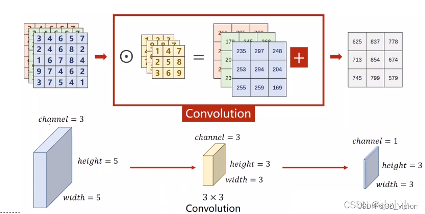
How to calculate the parameters of the model
First, assume that the size of the convolution kernel is K×K, there are C feature maps as input, the size of each output feature map is H×W, and the output is M feature maps.
Since the parameter quantity of the model is mainly composed of convolution, fully connected layer, BatchNorm layer and other parts, we take the parameter quantity of convolution as an example to calculate and analyze the parameter quantity: Convolution kernel parameter quantity: M×C×K×K,
partial Set parameter amount: M, overall parameter amount: M×C×K×K+M
The role of the fully connected layer
The fully connected layer maps the high-dimensional features learned by convolution to the label space, which can be used as the classifier module of the entire network.
Although there is redundancy in the parameters of the fully connected layer, it can still maintain a large model performance when the model performs migration learning.
At present, many models use global average pooling (GAP) instead of fully connected layers to reduce model parameters and still achieve SOTA performance.
The nature and common means of regularization?
Regularization is one of the core topics in machine learning. The essence of regularization is an operation that imposes a priori restrictions or constraints on a certain problem to achieve a specific purpose. In machine learning, we use regularization methods to prevent overfitting and reduce its generalization error.
Commonly used regularization methods: data enhancement, using L-norm constraints, dropout, early stopping, confrontation training
The characteristics of convolution
Convolution has three main characteristics:
1. Local connection. Compared with full connection, local connection will greatly reduce the parameters of the network.
2. Weight sharing. Parameter sharing can also reduce the overall parameter volume. The parameter weights of a convolution kernel are shared by the entire image, and the parameter weights in the convolution kernel will not be changed due to different positions in the image.
3. Downsampling. Downsampling can gradually reduce image resolution, reduce computing resource consumption, accelerate model training, and effectively control overfitting.
A summary of high-frequency interview questions at the BN level ( see here for details ):
The first is the role of the BN layer:
to pull all the data in a batch from an irregular distribution to a normal distribution. The advantage of this is that the data can be distributed in the sensitive area of the activation function. The sensitive area is the area with a large gradient, so the feedback error can be propagated faster during backpropagation.
What problem does the BN layer solve?
A classic assumption in statistical machine learning is that "the data distribution (distribution) of the source space (source domain) and the target space (target domain) are consistent". If they are inconsistent, then new machine learning problems such as transfer learning/domain adaptation will emerge. The covariate shift is a branch problem under the assumption of inconsistent distribution, which means that the conditional probabilities of the source space and the target space are consistent, but their marginal probabilities are different. For the output of each layer of the neural network, because they have undergone intra-layer operations, their distribution is obviously different from the distribution of the input signal corresponding to each layer, and the difference will increase as the network depth increases, but the label they can represent is still unchanged, which meets the definition of covariate shift.
Because the activation input value of the neural network before the nonlinear transformation deepens with the depth of the network, its distribution gradually shifts or changes (that is, the above-mentioned covariate shift). The reason why the training converges slowly is that the overall distribution gradually approaches the upper and lower limits of the nonlinear function (such as sigmoid), so this leads to the disappearance of the gradient of the low-level neural network during backpropagation, which is the training of the deep neural network. The essential reason for the slower and slower convergence ( the gradient is the rate at which the network weights learn in backpropagation ). And BN is to use a certain standardization method to forcibly pull the distribution of the input value of any neuron in each layer of neural network back to the standard normal distribution with a mean of 0 and a variance of 1, so as to avoid the gradient dispersion problem caused by the activation function. So rather than saying that the role of BN is to alleviate covariate shift, it can also be said that BN can alleviate the problem of gradient dispersion.
The difference between BN layer training and testing:
In the training phase, the BN layer standardizes each batch of training data, that is, uses the mean and variance of each batch of data. (The variance and standard deviation of each batch of data are different) (Using the full training set and variance is easy to overfit)
In the test phase, we generally only input one test sample, and there is no concept of batch. Therefore, the mean and variance used at this time are the mean and variance of the entire data set after training.
Why not use the mean and variance of the entire training set during BN training?
Because it is easy to overfit with the mean and variance of the entire training set, for BN, it is actually to standardize each batch of data to the same distribution, and the mean and variance of each batch of data will have a certain difference, not fixed This difference can increase the robustness of the model and reduce overfitting to a certain extent.
Where is the BN layer used?
In CNN, BN layers should be used in front of nonlinear activation functions. Since the input of the hidden layer of the neural network is the output of the nonlinear activation function of the previous layer, its distribution is still changing drastically in the early stage of training. At this time, restricting its first-order moment and second-order moment cannot well relieve Covariate Shift; while BN's The distribution is closer to a normal distribution, and limiting its first and second moments can make the distribution of values input to the activation function more stable.
Advantages and disadvantages of the BN layer Advantages
:
You can choose a larger initial learning rate. Because this algorithm converges very quickly.
You can use dropout, L2 regularization.
There is no need to use partial response normalization.
Datasets can be completely scrambled.
The model is more robust.
Disadvantages:
Batch Normalization is very dependent on the size of the Batch. When the Batch value is small, the calculated mean and variance are unstable.
So BN is not suitable for the following scenarios: small batch, RNN, etc. ,
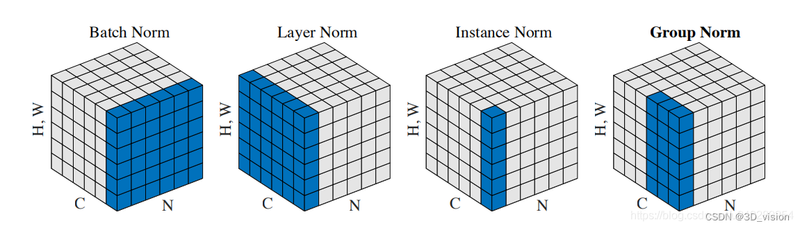
BN、LN、IN、GN:
Layer Nomalization
Instance Normalization
Group Normalization
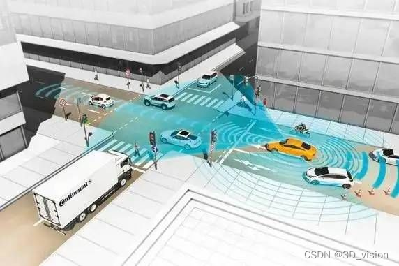
The principle of laser radar to obtain point cloud:
LiDAR emits a high-density laser beam, the beam travels in a straight line and hits the surface of the object, and then reflects back in the same direction (ignoring the diffraction phenomenon of a small amount of light), and the reflected light is detected and collected by a photodetector (photosensitive sensor). The 3D geometry of the object can be generated by combining the distance and direction information of the laser beam traveling back and forth. In actual use, the laser transmitter is placed on a continuously rotating base, so that the emitted laser beam can reach the surface of the object in different directions (front, back, left, right).
Summary of point cloud data processing:
Point cloud filtering
Point cloud filtering, as the name implies, is to filter out noise. The original collected point cloud data often contains a large number of hash points and isolated points.
The main methods of point cloud filtering are: bilateral filtering, Gaussian filtering, conditional filtering, straight-through filtering, random sampling consistent filtering, VoxelGrid filtering, etc. These algorithms are encapsulated in the PCL point cloud library.
Features and feature description
If a 3D point cloud is to be described, the location of the point cloud alone is not enough. It is often necessary to calculate some additional parameters, such as normal direction, curvature, textural features, and so on. Like the features of images, we need to describe the features of 3D point clouds in a similar way.
Commonly used feature description algorithms: normal and curvature calculation and eigenvalue analysis, PFH, FPFH, 3D Shape Context, Spin Image, etc.
PFH: point feature histogram descriptor, FPFH: cross-Su point feature histogram descriptor, FPFH is a simplified form of PFH.
Point cloud key points are extracted
on two-dimensional images. There are key point extraction algorithms such as Harris, SIFT, SURF, and KAZE, which extend the idea of feature points to three-dimensional space. Technically speaking, the number of key points is much smaller than the data volume of the original point cloud or image, and is combined with the local feature descriptor to form a key point descriptor to form a representation of the original data without losing representation. and descriptiveness, thereby speeding up the processing speed of subsequent identification, tracking and other data, the key point technology has become a very critical technology in 2D and 3D information processing.
There are several common 3D point cloud key point extraction algorithms: ISS3D, Harris3D, NARF, and SIFT3D.
These algorithms are all implemented in the PCL library, and the NARF algorithm is more common.
Point cloud registration
The concept of point cloud registration can also be compared to the registration in 2D images. Compared with 2D image registration, x, y, alpha, beta and other radiation change parameters are obtained, and 2D and 3D point cloud registration It can simulate the rotation and movement of a 3D point cloud, that is, a rotation matrix and a translation vector will be obtained, usually expressed as a 4×3 matrix, where 3×3 is the rotation matrix and 1 3 is the translation vector . Strictly speaking, there are 6 parameters, because the rotation matrix can also be transformed into a 1 3 rotation vector through the Rogrides transformation.
There are two commonly used point cloud registration algorithms: normal distribution transformation and the famous ICP point cloud registration. In addition, there are many other algorithms, listed as follows:
ICP: robust ICP, point to plane ICP, point to line ICP, MBICP, GICP
NDT 3D, Multi-Layer NDT
FPCS, KFPSC, SAC-IA
Line Segment Matching, ICL
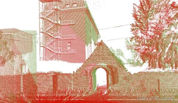
Point cloud classification and segmentation
The segmentation and classification processing of point cloud is much more complicated than the processing of two-dimensional images. Point cloud segmentation is divided into region extraction, line and surface extraction, semantic segmentation and clustering, etc. The same is the problem of segmentation. Point cloud segmentation involves too many areas. Generally speaking, point cloud segmentation is the basis of target recognition.
Segmentation: regional sound field, Ransac line-surface extraction, NDT-RANSAC, K-Means, Normalize Cut, 3D Hough Transform (line-surface extraction), connectivity analysis Classification: point-based classification, segmentation-based classification, supervised classification and unsupervised
classification .
The point cloud data obtained by 3D reconstruction
are all isolated points, and obtaining the entire surface from each isolated point is the problem of 3D reconstruction.
The directly collected point cloud is full of noise and isolated points. In order to reconstruct the surface, the 3D reconstruction algorithm often has to deal with this noise and obtain a smooth surface.
Commonly used 3D reconstruction algorithms and technologies include:
Poisson reconstruction, Delauary triangulatoins
surface reconstruction, human body reconstruction, building reconstruction, input reconstruction
real-time reconstruction: reconstruction of paper cups or dragon crops 4D growth table, human body posture recognition, expression recognition
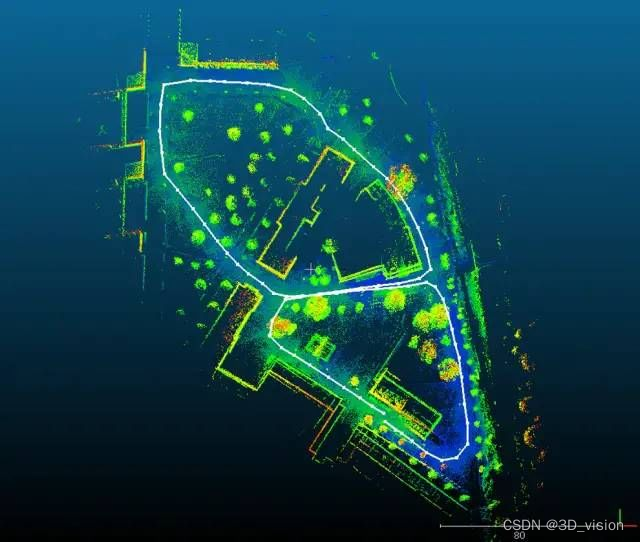
Point cloud datasets
The existing 3D point cloud datasets mainly include ModelNet40, ShapeNet, S3DIS, 3D Match, and KITTI. The first three are mainly used in CAD models, indoor building segmentation, and indoor scene registration. The KITTI dataset is mainly Applied to autonomous driving, ADAS, external scene vision SLAM, etc.
Deep Learning Method for Point Cloud Processing
At present, for the classification and segmentation of point cloud data, deep learning methods have become the mainstream. The more common ones are PointNet, PointNet++, DGCNN, PointCNN, PointSIFT, Point Transformer, and RandLANet, etc. Among them, the former two are mostly used.
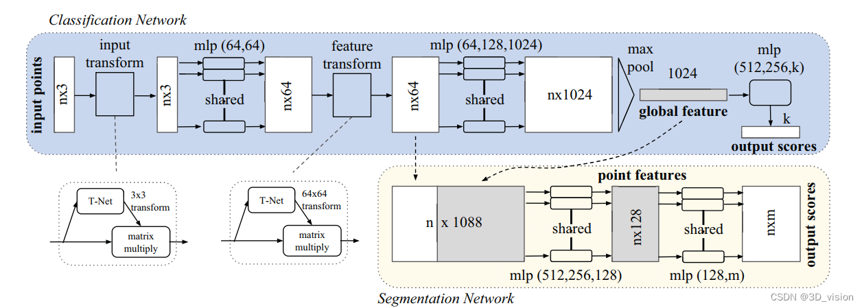
1. PointNet
 As can be seen from the figure, since the rotation of the point cloud is very simple, it only needs to multiply an N×D point cloud matrix by a D×D rotation matrix, so learn a 3× 3 matrix, it can be corrected; similarly, after the point cloud is mapped to the K-dimensional redundant space, the K-dimensional point cloud features are proofread again, but this proofreading needs to introduce a regularization penalty term, It is hoped that it is as close as possible to an orthogonal matrix.
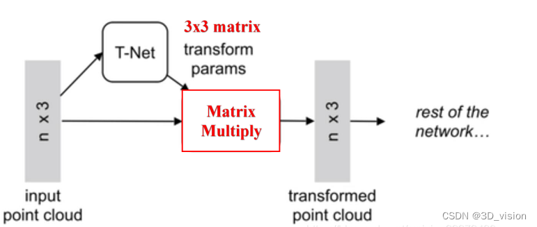
Specifically, for each N×3 point cloud input, corresponding to the 3D coordinate information of the original N points, the network first uses a T-Net to spatially align it (rotate to the front), where T-Net is Like a mini-point-net network, a 3×3 affine transformation matrix can be learned. Then map it to a 64-dimensional space through MLP, then align it, and finally map it to a 1024-dimensional space. At this time, for each point, there is a 1024-dimensional vector representation, and such a vector representation is obviously redundant for a 3-dimensional point cloud, so the maximum pooling operation is introduced at this time, and all 1024-dimensional channels are Only the largest one is kept, and the resulting 1×1024 vector is the global feature of the N point clouds.
If you are doing a classification problem, you can directly pass this global feature into the MLP to output the probability of each category; but if it is a segmentation problem, since you need to output point-by-point categories, it stitches the global features together. Based on the 64-dimensional point-by-point features of the point cloud, the network can use the geometry and global semantics of local and global features at the same time, and finally output the point-by-point classification probability through MLP.
2. PointNet++
From many experimental results, it can be seen that the segmentation effect of PointNet on the scene is very general. Because its network directly and violently pools all the points into a global feature, the connection between local points and points is not. learned by the network. In classification and Part Segmentation of objects, such problems can also be partially solved by centralizing the coordinate axes of objects, but in scene segmentation, this leads to very general effects.
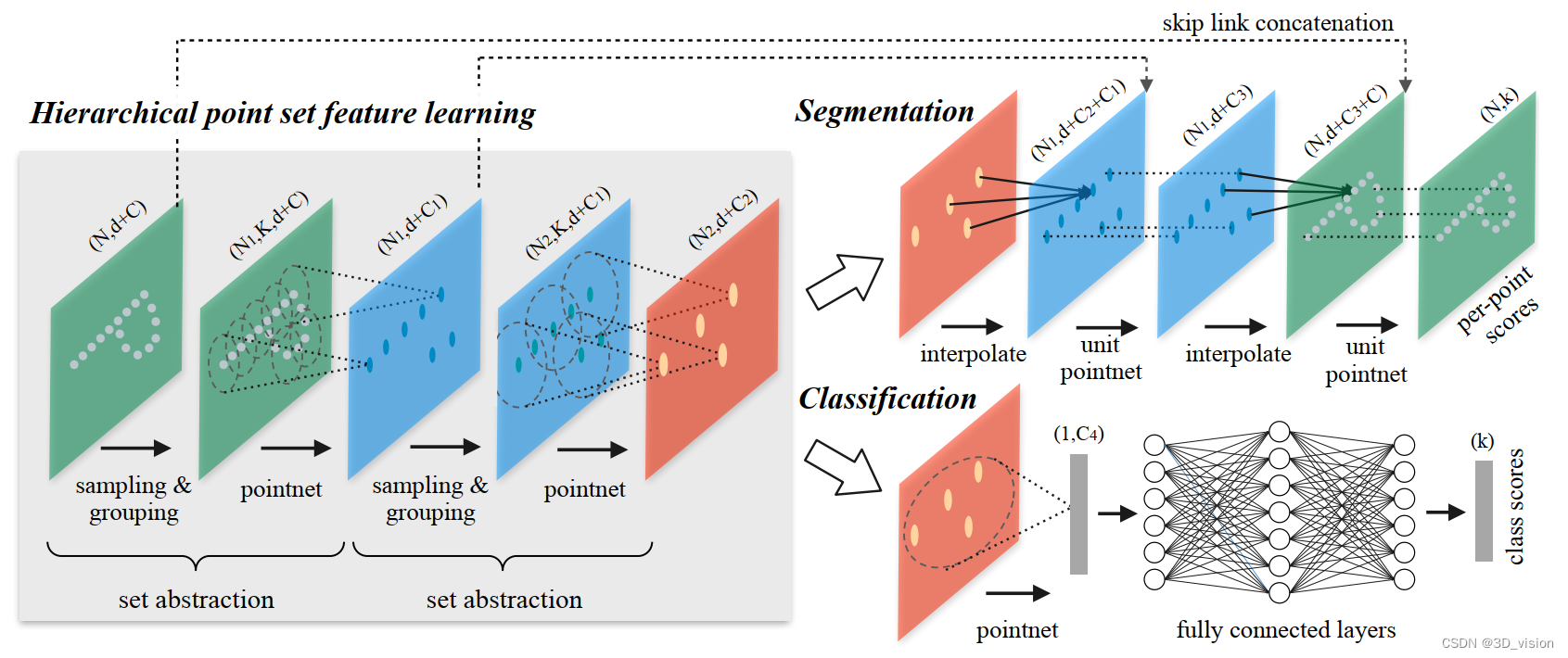
Further researchers proposed a hierarchical feature learning framework PointNet++ to solve this problem, thereby improving some limitations of PointNet. The hierarchical learning process is through a series of set levels of abstraction. Each collection abstraction level consists of a sampling group layer, grouping layer and PointNet layer. PointNet++ network structure
 PointNet++ mainly draws on the idea of CNN's multi-layer receptive field. CNN continuously uses the convolution kernel to scan the pixels on the image and do inner product by layering, so that the feature map has a larger receptive field, and each pixel contains more information. And PointNet++ imitates such a structure, as follows:
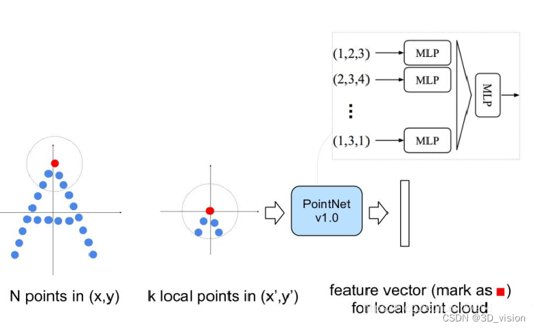
First, it takes a local sampling of the entire point cloud and draws a range, uses the points inside as local features, and uses PointNet to extract features once. Therefore, after many times of such operations, the number of original points becomes less and less, and each point is a local feature extracted by more points from the previous layer through PointNet, that is, each point Points contain more information. The article refers to such a layer as Set Abstraction.
A Set Abstraction mainly consists of three parts:
Sampling: use FPS (farthest point sampling) to randomly sample points
Grouping: use Ball Query to draw a circle with R as the radius, and use the point cloud in each circle as a cluster
PointNet: Local global feature extraction for point clouds after Sampling+Grouping
How to solve the problem of imbalance between positive and negative samples, and how to calculate the solution?
The focal loss loss function is usually used to solve the imbalance between positive and negative samples. This loss function reduces the weight of a large number of simple negative samples in training, which can also be understood as a kind of difficult sample mining.
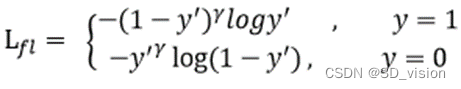
Focal loss is a modification based on the cross-entropy loss function. First, the two-category cross-entropy loss function is:

y is the output of the activation function, so it is between 0-1. It can be seen that for the normal cross-entropy loss function, for positive samples, the greater the output probability, the smaller the loss. For negative samples, the smaller the output probability, the smaller the loss. The loss function at this time is relatively slow in the iterative process of a large number of simple samples and may not be optimized to the optimum. So Focal loss improves binary cross-entropy:
first, it introduces the gama factor. When gama=0, it is the binary cross-entropy function. When gama>0, it will reduce the loss of easy-to-classify samples, making it more important to focus on difficult and wrong ones. points sample.
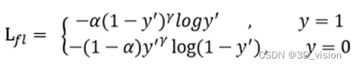
Then add the balance factor alpha to balance the uneven proportion of positive and negative samples. However, if only alpha is added, although the importance of positive and negative samples can be balanced, it cannot solve the problem of simple and difficult samples.
Point cloud key point extraction, feature description
ISS (Intrinsic Shape Signatures)
NARF
uniform sampling, voxel sampling
HARRIS
SIFT
SUSAN
AGAST
Common methods to improve the generalization ability of the model
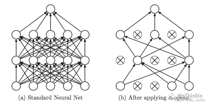
1. Dropout
first randomly deletes half of the hidden neurons in the network, and the input and output neurons remain unchanged. Then the input x is forward-propagated through the modified network, and then the obtained loss result is back-propagated through the modified network. After performing this process on a small batch of training samples, update the corresponding parameters (w, b) on the neurons that have not been deleted according to the stochastic gradient descent method, and then continue to repeat this process.
Dropout is simply the random deactivation of model nodes, so that it does not depend too much on some local characteristics of the data.
2. Adding a regular term to the loss function of the regularized
model can prevent the parameters from being too large, prevent overfitting and improve the generalization ability.
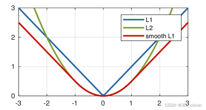
L1 loss, L2 loss, smooth L1 loss principle and difference
First, post the images of these loss functions:
L1 loss:
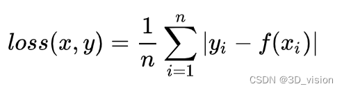
Among them, yi is the real value, f(xi) is the predicted value, and n is the number of sample points
Advantages and disadvantages:
Advantages: No matter what kind of input value, there is a stable gradient, which will not cause the gradient explosion problem, and has a more robust solution. Disadvantages: The
center point is an inflection point, and the derivative cannot be obtained. If the gradient descends just right After learning w=0, there is no way to continue
When to use it?
The regression task
is simple.
The neural network is usually more complicated. It is rare to directly use L1 loss as the loss function.
L2 loss:
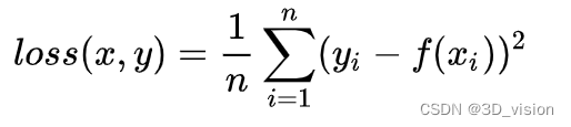
Among them, yi is the real value, f(xi) is the predicted value, and n is the number of sample points
Advantages and disadvantages:
Advantages: all points are continuous and smooth, convenient for derivation, and have a relatively stable solution
Disadvantages: not particularly robust, because when the input value of the function is far from the real value, the corresponding loss value is large on both sides, When using the gradient descent method to solve the problem, the gradient is very large, which may lead to a gradient explosion
When to use it?
The numerical characteristics of the regression task
are not large (to prevent the loss from being too large, which will cause the gradient to be large and the gradient
will explode).
Smooth L1 loss
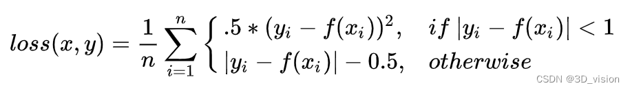 analysis, when the difference between the predicted value f(xi) and the actual value yi is small (the absolute value difference is less than 1), the L2 loss is actually used; when the difference is large, the translation of the L1 loss is used. Therefore, Smooth L1 loss is actually a combination of L1 loss and L2 loss, and has some advantages of both:
when the difference between the real value and the predicted value is small (the absolute value difference is less than 1), the gradient will also be relatively small (the loss function is larger than the normal L1 The loss is more smooth here)
When the difference between the real value and the predicted value is large, the gradient value is small enough (the gradient value of ordinary L2 loss is very large in this position, and the gradient is easy to explode)
When to use it? Larger values in
the regression task feature are suitable for most problems (used the most!)
The difference between the three:
(1) L1 loss is not smooth at the zero point, and it cannot be guided here, so when w=0, it cannot continue the gradient descent, and it is less used
(2) L2 loss is more sensitive to outliers, outliers The gradient at the point is very large, and it is easy to explode the gradient
(3) smooth L1 loss combines the advantages of L1 and L2, modifies the problem of non-smoothness at zero point, and is more robust to outliers than L2 loss
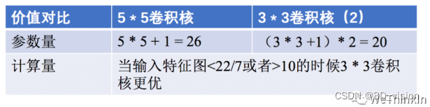
The impact of replacing the 5 5 convolution kernel with two cascaded 3 3 convolution kernels on parameters and calculations ( reference )
A large-size convolution kernel can bring a larger receptive field, but also means more parameters: what is the benefit of
using 3 3 instead of 5 5?
1. Increase the number of network layers, and activation functions can be added between layers, which increases the nonlinear expression ability of the network.
2. If the channel of the convolution kernel is 1, then two 3*3 convolution kernels have 18 parameters, and one 5*5 convolution kernel has 25 parameters (normally, the number of channels should also be considered).
Common gradient descent methods and principles
First a little about gradient descent :
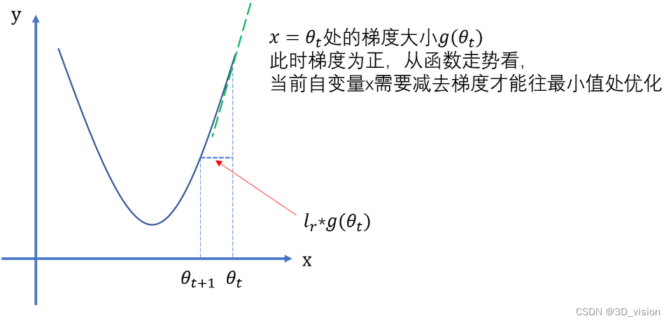
the gradient is a vector that tells us the direction of the weights. More precisely, it tells us how to change the weights so that the loss changes the fastest. We call this process gradient descent because it uses gradients to bring the loss curve down to a minimum.
If we can successfully train a network to do this, its weights must somehow represent the relationship between these features and the objects represented in the training data. Besides the training data, we need two more things:
A "loss function" that measures how well the network's predictions are.
An "optimizer" that tells the network how to change its weights.
Common "optimizers" are: SGD, Adam, BGD, momentum, Adagrad, NAG, ( the difference between SGD and Adam )
because I use SGD in my project, so I will focus on this:
SGD: Stochastic gradient descent:
use samples Some of the examples in are used to approximate all samples to adjust, so stochastic gradient descent will bring certain problems, because the calculated gradient is not an accurate one, and it is easy to fall into a local optimal solution.
Dynamic adjustment of learning rate LR for deep learning
1. What is the learning rate:
the deep network model is trained on an unknown and complex function with a large number of parameters. The purpose of training is to find a set of optimal parameters. The learning rate lr controls the speed of parameter update, and The speed at which the model learns.
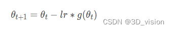
where θ t + 1 is the parameter value after the t + 1 iteration, θ t is the parameter value after the t iteration, lr is the learning rate, g ( θ t ) is the parameter θ calculated at the t iteration The obtained gradient value.
 2. Why should the learning rate be adjusted dynamically?
Because the network needs to speed up the convergence in the right direction at the beginning, but it will converge slowly when it is close to the target, so the learning rate must be adjusted dynamically.
3. The method and
principle of dynamically adjusting the learning rate Portal
3.1 lr_scheduler.LambdaLR
3.2 lr_scheduler.StepLR
3.3 lr_scheduler.MultiStepLR
3.4 lr_scheduler.ExponentialLR
3.5 lr_scheduler.CosineAnnealingLR
3.6
lr_scheduler.ReduceLR7CyPlateau_schedlic 3
The difference between concat and add in neural network
How to understand the way of concat and add to fuse features:
In each network model, ResNet, FPN, etc. use element-wise add to fuse features, while DenseNet, etc. use concat to fuse features.
concat is an increase in the number of channels.
add is the addition of feature maps, and the number of channels remains unchanged.
How to understand? :
add means that the amount of information under the characteristics of the description image has increased, but the dimension of the description image itself has not increased, but the amount of information under each dimension has increased, which is obviously beneficial to the classification of the final image.
concat is the combination of the number of channels, that is to say, the number of features (the number of channels) describing the image itself has increased, while the information under each feature has not increased.
The calculation amount of add is much smaller than that of concat.
Examples of concat and add:
For example, Densenet using concat:
advantages:
(1) solves the problem of gradient disappearance in deep networks
(2) strengthens the propagation of features
(3) encourages feature reuse
(4) reduces model parameters
(5) ) can reduce the overfitting problem of small samples
Disadvantages:
very memory consumption
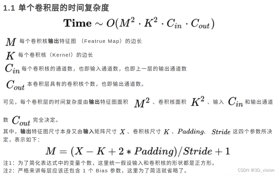
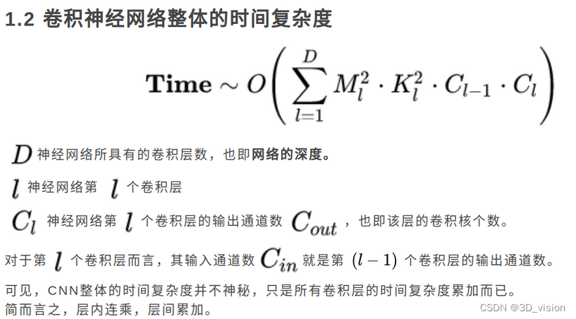
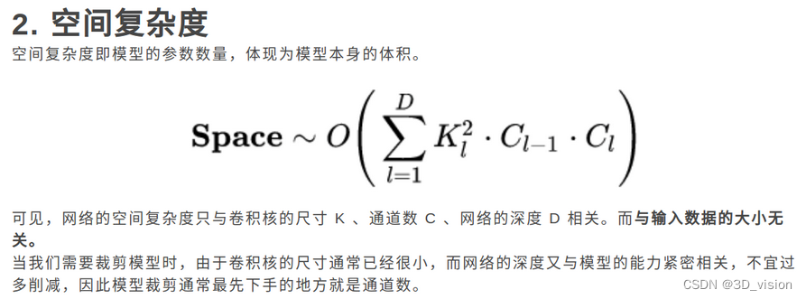
How to calculate the convolution time complexity and space complexity of convolutional neural network:
Post a picture, too lazy to write, you can click here for details
Related concepts and calculations of NMS in target detection
In target detection, we can use non-maximum suppression (NMS) to post-process a large number of generated candidate boxes to 去除冗余的候选框obtain the most representative results to speed up the efficiency of target detection.

Non-Maximum Suppression (NMS) process:
1. First, we need to set two values: a Score threshold and an IOU threshold.
2. For each type of object, traverse all candidate boxes of this class, filter out candidate boxes with a Score value lower than the Score threshold, and sort according to the category classification probability of the candidate boxes: A < B < C < D < E < F.
3. First mark the maximum probability rectangular frame F as the candidate frame we want to keep.
4. Starting from the rectangular frame F with the highest probability, judge whether the intersection-over-union ratio (IOU) of A~E and F is greater than the IOU threshold. Assuming that the overlapping degree of B, D and F exceeds the IOU threshold, then remove B and D.
5. From the remaining rectangular boxes A, C, and E, select E with the highest probability and mark it as a candidate box to be retained, then judge the degree of overlap between E and A, C, and remove rectangles whose overlap exceeds the set threshold frame.
6. Repeat this until the remaining rectangles are gone, and mark all the rectangles that you want to keep.
7. After each category is processed, return to step 2 to process the next category of objects again.
How to deal with unbalanced data categories?
1. Data augmentation.
2. Sampling is done for minority category data, and undersampling is done for majority category data.
3. The weight balance of the loss function. (Different categories have different loss weights, and the best parameters need to be adjusted manually)
4. Collect more data from minority categories.
5. Transform the definition of the problem, and transform the problem into an outlier detection or trend detection problem. Outlier detection is to identify those rare events, and change trend detection is different from outlier detection, which recognizes by detecting unusual change trends.
6. Use new evaluation metrics.
7. Threshold adjustment, adjust the original default threshold of 0.5 to: fewer categories/(less categories + more categories).
What is the bias and variance of the model?
Error (Error) = bias (Bias) + variance (Variance) + noise (Noise), generally, we call the difference between the predicted output of the machine learning model and the real label of the sample as error, which reflects the entire model the accuracy.
Noise: Describes what any machine learning algorithm can achieve on the current task 期望泛化误差的下界, that is, it describes the difficulty of the nature of the current task.
Bias: It measures the ability of the model to fit the training data. The bias reflects all the models trained by all the sampled training sets of the same size, that is, the model 输出平均值和真实label之间的偏差itself 精确度.
Bias is usually caused by our wrong assumptions about the machine learning algorithm, such as the real data distribution maps to a quadratic function, but we assume that the model is a linear function.
The smaller the bias (Bias), the stronger the fitting ability (may cause overfitting); conversely, the weaker the fitting ability (may cause underfitting). The larger the deviation, the more it deviates from the real data.
Variance describes the range of variation of the predicted value, the degree of dispersion, that is, the distance from the expected value. 方差越大,数据的分布越分散,模型的稳定程度越差.
The variance also reflects the error between each output of the model and the expected output of the model, that is, the stability of the model. The error introduced by the variance is usually reflected in the increment of the test error relative to the training error.
Variance is usually caused by the complexity of the model being too high relative to the number of training samples. 方差越小,模型的泛化能力越高;反之,模型的泛化能力越低.
If the fitting effect of the model on the training set is relatively good, but the fitting effect on the test set is relatively poor, it means that the variance is large, indicating that the stability of the model is poor. This phenomenon may be due to the model overfitting the training set. combined.
What types of features are extracted at different levels of convolution?
Shallow convolution --> extract edge features
Middle convolution --> extract local features
Deep convolution --> extract global features
How to choose the convolution kernel size?
The most commonly used is a 3 3 convolution kernel, two 3 3 convolution kernels and a 5 5 convolution kernel have the same receptive field, but reduce the amount of parameters and calculations, and speed up model training. At the same time, due to the increase of the convolution kernel, the nonlinear expression ability of the model is greatly enhanced.
However, large convolution kernels (7 7, 9*9) also have room for use, and there are still many applications in GAN, image super-resolution, image fusion and other fields.
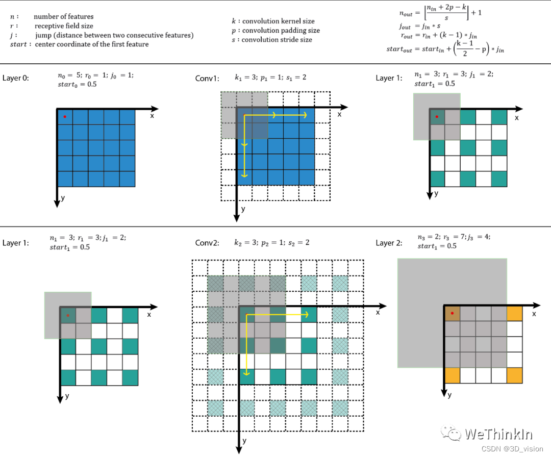
Related concepts of convolution receptive field
Many models of target detection and target tracking use the RPN layer. The anchor is the basis of the RPN layer, and the receptive field (RF) is the basis of the anchor.
The role of the receptive field:
1. Generally speaking, the larger the receptive field, the better. For example, the receptive field of the last convolutional layer in the classification task should be larger than the input image.
2. When the receptive field is large enough, less information is ignored.
3. In the target detection task, set the anchor to align with the receptive field. If the anchor is too large or deviates from the receptive field, the performance will be affected to a certain extent.
Receptive field calculation:
 method of increasing receptive field:
1. Use hole convolution
2. Use pooling layer
3. Increase convolution kernel
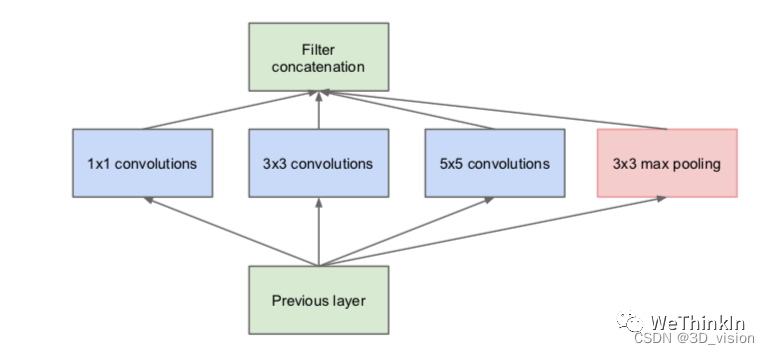
Can each layer of the network use only one size of convolution kernel?
Conventional neural networks generally use only one size convolution kernel per layer, but the feature maps of the same layer can be separated 使用多个不同尺寸的卷积核,以获得不同尺度的特征, and then these features are combined, and the obtained features are often better than those using a single size convolution kernel, such as GoogLeNet, Inception The series of networks use multiple different convolution kernel structures for each layer. As shown in the figure below, the input feature map passes through three convolution kernels of 1 1 , 3 3 , and 5*5 in the same layer, and then integrates the respective feature maps. The new features obtained can be regarded as different feelings. The combination of features extracted from the field will have stronger expressive power than a single-size convolution kernel.
What is the role of 1*1 convolution?
The main functions are as follows:
1. Realize the interaction and integration of feature information.
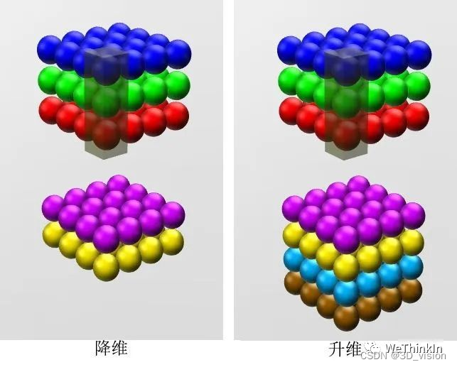
2. The number of feature map channels is increased and reduced, and the number of parameters can be reduced during dimensionality reduction.
3. 1*1 convolution + activation function --> can increase nonlinearity and improve the expressive ability of the network.
1*1 convolution was first used in NIN (Network in Network), and it was later used in networks such as GoogLeNet and ResNet.
The role of the fully connected layer?
The fully connected layer maps the high-dimensional features learned by convolution to the label space, which can be used as the classifier module of the entire network.
At present, many models use global average pooling (GAP) instead of fully connected layers to reduce model parameters and still achieve SOTA performance.
Insert a basic knowledge point here:
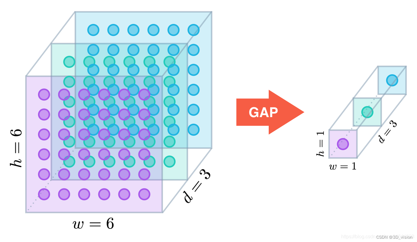
global average pooling (GAP) converts multidimensional matrices into feature vectors through pooling operations to replace full connections (FC).
Advantages:
1. A large number of parameters in FC are reduced, making the model more robust and resistant to overfitting. Of course, underfitting may also occur.
2. GAP transitions between feature maps and final classification more naturally.
The working principle of GAP is shown in the figure below:
Insert one more:
为什么使用全局平均池化代替全连接层后,网络的收敛速度会变慢?
1. For the model with CNN+FC structure, for the training process, the learning pressure of the whole model is mainly concentrated on the FC layer (the parameter quantity of the FC layer accounts for 80% of the total model parameter quantity), at this time, the features learned by the CNN layer are more Tend to low-level general-purpose features. Even if the features learned by the CNN layer are relatively low-level, the powerful FC layer can also achieve good classification by learning and adjusting parameters. 2.
CNN+GAP structure model, because GAP is used instead of FC, the model The number of parameters of the model decreases sharply. At this time, the learning pressure of the model is all forwarded to the CNN layer. Compared with the CNN+FC layer, the CNN layer at this time not only needs to learn the general features of the lower layer, but also learns more advanced classification features. , learning becomes more difficult and network convergence becomes slower
But: In summary, although the global average pooling instead of the fully connected layer can reduce the number of parameters of the model and prevent the model from overfitting, but, 不利于模型的迁移学习because CNN+GAP的结构使得很多参数“固化”在卷积层中when adding a new classification, it means that a considerable number of convolutional layer features need Re-adjustment (more difficult to learn); and the fully connected layer can better perform migration learning, because a large part of its parameter adjustment is in the fully connected layer, although the parameters of the convolutional layer will also be adjusted during migration , but relatively much smaller
The role of pooling in CNN?
The role of the pooling layer 是对感受野内的特征进行选择,提取区域内最具代表性的特征,能够有效地减少输出特征数量,进而减少模型参数量。is usually divided into Max Pooling, Average Pooling and Sum Pooling according to the type of operation. They respectively extract the maximum, average and sum of the feature values in the receptive field as Output, the most commonly used are max pooling and average pooling.
What methods can improve the generalization ability of CNN model?
1. Collect more data: The data determines the upper limit of the algorithm.
2. Optimize data distribution: data category balance.
3. Choose an appropriate objective function.
4. Design an appropriate network structure.
5. Data enhancement.
6. Weight regularization.
7. Use an appropriate optimizer, etc.
What is the difference between One-stage target detection and Two-stage target detection?
Two-stage目标检测算法: First perform region generation (region proposal, RP) (a pre-selection box that may contain the object to be inspected), and then classify the samples through the convolutional neural network. Its precision is higher, but its speed is slower.
Main logic: feature extraction --> generate RP --> classification/positioning regression.
Common Two-stage target detection algorithms include: Faster R-CNN series and R-FCN.
One-stage目标检测算法: Without RP, directly extract features from the network to predict object classification and location. Its speed is faster, and its accuracy is slightly lower than that of the Two-stage algorithm.
Main logic: feature extraction -> classification/positioning regression.
Common one-stage target detection algorithms include: YOLO series, SSD and RetinaNet, etc.
What methods can improve the effect of small target detection?
1. Improve image resolution. Small objects may only contain a few pixels in the bounding box, so the feature richness of small objects can be increased by increasing the resolution of the image.
2. Improve the input resolution of the model. This is a general method with better results, but it will cause the problem of slowing down the speed of model inference.
3. Tile the image.
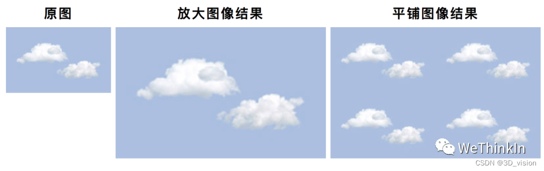 4. Data enhancement. Small object detection enhancements include random cropping, random rotation, and mosaic enhancement, etc.
5. Automatically learn the anchor.
6. Category optimization.
The characteristics of the ResNet model and the problems it solves?
The characteristic of the model is the designed residual structure, which is very sensitive to small changes in the model output.
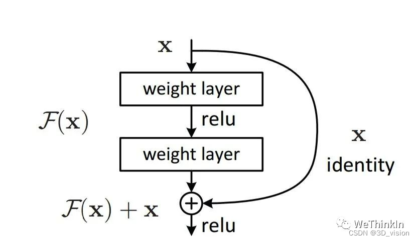
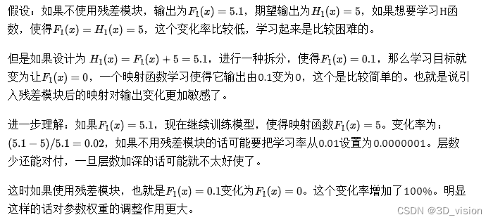
Why is adding the residual module effective?
I took a screenshot directly:
What is overfitting, and what are the methods to solve it?
过拟合: The model fits well on the training set, but the model even learns the characteristics of the noise data, and loses the generalization ability to the test set.
解决过拟合的方法:
1. Re-clean the data. Impurity of the data will lead to over-fitting. In this case, the data needs to be re-cleaned or re-selected.
2. Increase the number of training samples. Using more training data is the most effective way to solve overfitting. We can expand the training data through certain rules. For example, in the image classification problem, we can expand the data through image translation, rotation, scaling, adding noise, etc.; we can also use the GAN network to synthesize a large amount of new training data.
3. Reduce the complexity of the model. Appropriately reducing the model complexity can prevent the model from fitting too much noise data. Reduce the number of network layers, the number of neurons, etc. in the neural network.
4. Add a regularization method to increase the coefficient of the regularization term. Add certain regular constraints to the parameters of the model, such as adding the weight value to the loss function.
5. The dropout method is adopted. The dropout method is to deactivate neurons with a certain probability during training.
6. Early stopping to reduce the number of iterations.
7. Increase the learning rate.
8. Integrated learning method. Integrated learning is to integrate multiple models together to reduce the risk of overfitting of a single model, such as the Bagging method.
What is underfitting and what are the ways to solve it?
欠拟合: The effect of the model on the training set and the test set is not good. The root cause is that the model has not learned the characteristics of the data set.
解决欠拟合的方法:
1. It can increase the complexity of the model. For neural networks, the number of network layers or the number of neurons can be increased.
2. Reduce the regularization coefficient. The purpose of regularization is to prevent overfitting, but now that the model is underfitting, it is necessary to reduce the regularization coefficient in a targeted manner.
The nature of regularization and common regularization methods?
Regularization is one of the core topics in machine learning. 正则化本质是对某一问题加以先验的限制或约束以达到某种特定目的的一种操作。In machine learning, we use regularization methods to prevent overfitting and reduce its generalization error.
Commonly used regularization methods:
1. Data enhancement
2. Use L-norm constraints
3. Dropout
4. Early stopping
5. Adversarial training
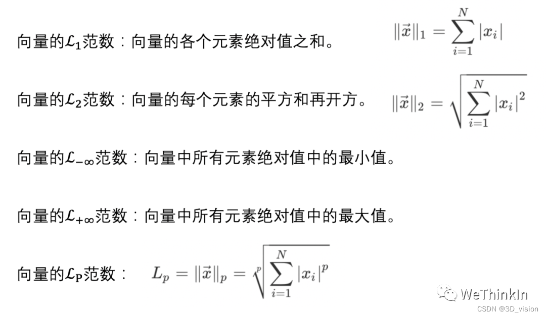
The role of the L norm?
The L norm mainly plays the role of regularization ( 即用一些先验知识约束或者限制某一抽象问题), and regularization is mainly to prevent the model from overfitting.
The norm is mainly used to represent the distance in high-dimensional space, so in some generation tasks, the L norm is also directly used to measure the difference between the generated image and the original image.
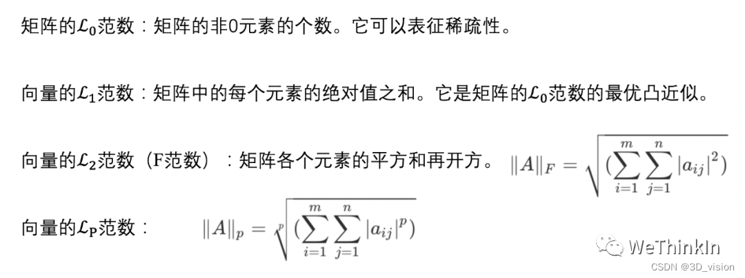
The norms in deep learning are listed below:
The role of dropout?
Dropout is to deactivate neurons with a certain probability during the training process, that is, the output is equal to 0. Thereby improving the generalization ability of the model and reducing overfitting.
We can understand intuitively from two aspects Dropout的正则化效果:
1) During each round of Dropout training 随机丢失神经元的操作相当于多个模型进行取平均, it has the effect of vote when used for prediction.
2) Reduce the complex co-adaptation between neurons. 当隐藏层神经元被随机删除之后,使得全连接网络具有了一定的稀疏化, thus effectively mitigating the synergistic effect of different features. That is to say, some features may depend on the joint action of hidden nodes with fixed relationships, and through Dropout, it can effectively avoid the situation that some features are only effective in the presence of other features, increasing the robustness of the neural network. Stickiness.
Dropout在训练和测试时的区别: Dropout only works during training. It is to reduce the dependence of neurons on some upper layer neurons. It is similar to integrating multiple models with different network structures to reduce the risk of overfitting. When testing, the entire trained model should be used, so Dropout is not required.
Definition and function of Softmax activation function
In the binary classification problem, we can use the sigmoid function to map the output to the [0, 1] interval to obtain the probability of a single class. When we generalize the problem to a multi-classification problem, we can use the Softmax function to map the output value to a probability value.
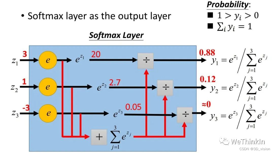
It is defined as:
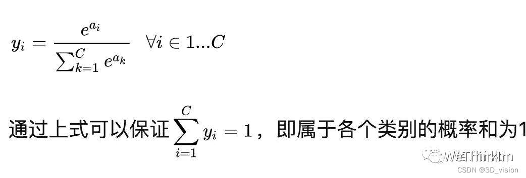
where a represents the output of the model.
Definition and function of cross entropy
Cross entropy (cross entropy) is often used in classification tasks in deep learning, which can represent the gap between the predicted value and the ground truth.
Cross entropy is a concept in information theory. It is defined as:

P represents the probability distribution of gt, and q represents the probability distribution of the predicted value. Cross entropy evolves from relative entropy (KL divergence), log represents the amount of information, and the larger q means the greater the possibility and the greater the amount of information. Through continuous training and optimization, the value of the cross-entropy loss function is gradually reduced to achieve the purpose of reducing the distance between p and q.
Calculation of model parameters:
First, assume that the size of the convolution kernel is K×K, there are C feature maps as input, the size of each output feature map is H×W, and the output is M feature maps.
Since the parameter quantity of the model is mainly composed of convolution, fully connected layer, BatchNorm layer and other parts, we take the parameter quantity of convolution as an example to calculate and analyze the parameter quantity:
Convolution kernel parameters: M×C×K×K
Bias parameter amount: M
Overall parameter quantity: M×C×K×K+M
Interpolation algorithm commonly used in model training?
Commonly used interpolation algorithms for resize images during model training are: nearest neighbor interpolation, bilinear interpolation, and bicubic interpolation.
最近邻插值: The influence of other adjacent pixels is not considered, so the gray value has obvious discontinuity after resampling, the image quality is greatly lost, and there are mosaics and aliasing.
双线性插值: Also called first-order interpolation, it uses the correlation between the four nearest neighbor pixels of the pixel to be sought in the source image, and obtains the value of the pixel to be sought through two linear interpolations.
双三次插值: Also called cubic convolution interpolation, it utilizes the values of 16 adjacent pixels in the source image, that is, the weighted average of these 16 pixels.
Common image preprocessing operations?
Generally, the data is first normalized (Normalization) processing [0, 1], and then the standardization (Standardization) operation is performed, and the data is converted into one by using the theorem of large numbers, and finally 标准正态分布some data enhancement processing is performed.
归一化后,可以提升模型精度. The features between different dimensions are numerically comparable, which can greatly improve the accuracy of the classifier. 标准化后,可以加速模型收敛. The optimization process of the optimal solution will obviously become smoother, and it is easier to correctly converge to the optimal solution.
The concept and simple derivation of the backpropagation algorithm (BP)
反向传播(Backpropagation,BP)算法是一种与最优化方法(如梯度下降法)结合使用的,用来训练人工神经网络的常见算法。The BP algorithm calculates the gradient of the loss function for all weights in the network, and feeds the gradient back to the optimization method to update the weights to minimize the loss function.该算法会先按前向传播方式计算(并缓存)每个节点的输出值,然后再按反向传播遍历图的方式计算损失函数值相对于每个参数的偏导数。
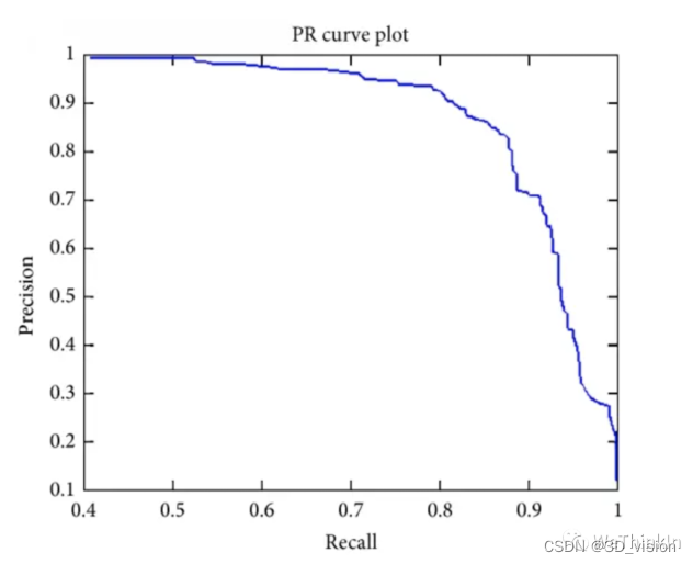
The meaning of AP, AP50, AP75, mAP and other indicators in target detection
AP: Area under the PR curve.
AP50: The AP value when the fixed IoU is 50%.
AP75: The AP value when the fixed IoU is 75%.
AP@[0.5:0.95]: The value of IoU is divided every 5% from 50% to 95%, and the 10 groups of AP values are averaged.
mAP: Calculate the AP for all categories, and then take the average.
mAP@[.5:.95] (i.e. mAP@[.5,.95]): indicates different IoU thresholds (from 0.5 to 0.95, step size 0.05) (0.5, 0.55, 0.6, 0.65, 0.7, 0.75, 0.8, 0.85, 0.9, 0.95) on average mAP .
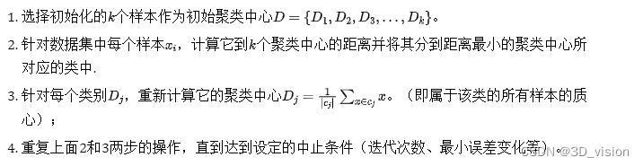
K-means algorithm logic?
The K-means algorithm 一个实用的无监督聚类算法,其聚类逻辑依托欧式距离,当两个目标的距离越近,相似度越大。divides a given sample set into K clusters according to the distance between samples. Let the points in the cluster be connected as closely as possible, and make the distance between the clusters as large as possible.
The main algorithm steps of K-Means:
The main advantages of K-Means:
1. Simple principle, easy implementation, and fast convergence.
2. The clustering effect is better
3. The interpretability of the algorithm is relatively strong
4. The main parameter that needs to be adjusted is the number of clusters k
The main disadvantages of K-Means:
1. The K value needs to be set manually, which is difficult to grasp.
2. It is sensitive to the initial cluster center, and different selection methods will get different results.
3. It is difficult to converge for non-convex data sets.
4. If the data of each hidden category is unbalanced, for example, the amount of data of each hidden category is seriously unbalanced, or the variance of each hidden category is different, the clustering effect is not good.
5. The iteration result is only a local optimum.
6. Sensitive to noise and abnormal points.
K nearest neighbor algorithm logic?
K-nearest neighbor (K-NN) algorithm 计算不同数据特征值之间的距离进行分类. There is a sample data set, also called a training data set, and each data in the data set has a label, that is, we know the mapping relationship between each data and its category. Then, after inputting new data without labels, find the K data closest to the new data in the training data set, and then extract the label that is the majority of the K data as the label of the new data ( ) 少数服从多数逻辑.
The main steps of the K nearest neighbor algorithm:
- Calculate the distance between the new data and each training data.
- Sort by increasing distance.
- Select the K points with the smallest distance.
- Determine the frequency of occurrence of the category of the first K points.
- Return the class with the highest frequency among the top K points as the predicted class for new data.
The results of the K-nearest neighbor algorithm largely depend on the choice of K. The distance calculation generally uses classic distance measures such as Euclidean distance or Manhattan distance.
The main advantages of the K nearest neighbor algorithm:
- The theory is mature and the thinking is simple, which can be used for both classification and regression.
- Can be used for non-linear classification.
- There are no assumptions about the data, high accuracy, and insensitive to outliers.
- It is more suitable for scenarios with a relatively large amount of data, and those scenarios with a relatively small amount of data are more prone to misclassification when using the K-nearest neighbor algorithm.
The main disadvantages of the K nearest neighbor algorithm:
- High computational complexity; high space complexity.
- When the samples are unbalanced, the prediction accuracy for rare categories is low.
- It is a lazy learning method, basically no learning, resulting in slower prediction speed than algorithms such as logistic regression.
- Not very interpretable.
3D point cloud data processing method
1. Point cloud filtering (data preprocessing)
Point cloud filtering, as the name implies, is to filter out noise.
The main methods of point cloud filtering are: bilateral filtering, Gaussian filtering, conditional filtering, straight-through filtering, random sampling consistent filtering, VoxelGrid filtering, etc. These algorithms are encapsulated in the PCL point cloud library.
2. Point cloud key points
We all know that on two-dimensional images, there are key point extraction algorithms such as Harris, SIFT, SURF, and KAZE. The idea of this feature point can be extended to three-dimensional space. Technically speaking, the number of key points is much smaller than the data volume of the original point cloud or image, and combined with the local feature descriptor, the key point descriptor is often used to form the representation of the original data without losing the representation. and descriptiveness, thereby speeding up the processing speed of subsequent recognition, tracking and other data, therefore, the key point technology has become a very critical technology in 2D and 3D information processing.
There are several common 3D point cloud key point extraction algorithms: ISS3D, Harris3D, NARF , SIFT3D
3. Features and feature description
If a 3D point cloud is to be described, the position of the point cloud alone is not enough, and some additional parameters, such as normal direction, curvature, textural features, etc., need to be calculated. Like the features of images, we need to describe the features of 3D point clouds in a similar way.
Commonly used feature description algorithms include: normal and curvature calculation, eigenvalue analysis, PFH, FPFH, 3D Shape Context, Spin Image, etc.
PFH: point feature histogram descriptor, FPFH: cross-Su point feature histogram descriptor, FPFH is a simplified form of PFH.
4. Point cloud registration
The concept of point cloud registration can also be compared to registration in 2D images, except that the 2D image registration obtains radiation change parameters such as x, y, alpha, beta, etc., and point cloud registration The standard can be simulated as the movement and alignment of a 3D point cloud, that is, a rotation matrix and a translation vector will be obtained, usually expressed as a 4×3 matrix, where 3×3 is the rotation matrix and 1×3 is the translation vector. Strictly speaking, there are 6 parameters, because the rotation matrix can also be transformed into a 1×3 rotation vector through the Rogrides transformation.
There are two commonly used point cloud registration algorithms: normal distribution transformation and the famous ICP point cloud registration . In addition, there are many other algorithms, listed as follows:
ICP: robust ICP, point to plane ICP, point to line ICP, MBICP, GICP
NDT 3D, Multi-Layer NDT
FPCS, KFPSC, SAC-IA
Line Segment Matching, ICL
5. Segmentation and classification of point cloud
Segmentation and classification of point cloud can be regarded as a big topic. Here, there are many problems compared with two-dimensional images because of the addition of one dimension. Point cloud segmentation is divided into area extraction, line and surface extraction, Semantic segmentation and clustering, etc. The same is the problem of segmentation. Point cloud segmentation involves too many aspects, and it is indeed unclear in a few words. Only understand it literally, and then classify it when encountering specific problems. Generally speaking, point cloud segmentation is the basis of object recognition .
Segmentation: Regional sound field, Ransac line-surface extraction, NDT-RANSAC, K-Means, Normalize Cut, 3D Hough Transform (line-surface extraction), connectivity analysis Classification: Point-based classification, segmentation-based classification, supervised classification and unsupervised
classification
6. SLAM graph optimization
SLAM is another big topic. In SLAM technology, the point cloud data is mainly obtained at the front end of the image, while the optimization at the back end mainly relies on graph optimization tools. The development of SLAM technology in recent years has also changed this technical strategy. In the past classic strategies, in order to solve the LandMark and Location and convert it into a sparse graph optimization, the g2o tool is often used for graph optimization. Below are some commonly used tools and methods.
g2o, LUM, ELCH, Toro, SPA
SLAM methods: ICP, MBICP, IDC, likehood Field, Cross Correlation, NDT
7. Target recognition and retrieval
This is an application-level problem in point cloud data processing. Simply put, Hausdorff distance is often used for target recognition and retrieval of depth maps. Now many 3D face recognition uses this technology to do.
8. Change detection
When the unordered point cloud is continuously changing, the octree algorithm is often used to detect changes. This algorithm needs to be combined with the key point extraction technology. The octree algorithm is also a classic among the classics.
9. 3D reconstruction
The point cloud data we obtained are all isolated points, how to get the whole surface from each isolated point, this is the topic of 3D reconstruction.
When playing kinectFusion, if we don't understand, we will find that the surface gradually becomes smoother, which is the effect of the continuous iteration of the reconstruction algorithm. The point cloud we collected is full of noise and isolated points. In order to reconstruct the surface, the 3D reconstruction algorithm often has to deal with this noise and obtain a surface that looks very comfortable.
Commonly used 3D reconstruction algorithms and technologies include:
Poisson reconstruction, Delauary triangulatoins
surface reconstruction, human body reconstruction, building reconstruction, input reconstruction
Real-time reconstruction: reconstruction of paper cup or dragon crop 4D growth table, human body posture recognition, expression recognition
10. Point cloud data management
Point cloud compression, point cloud index (KDtree, Octree), point cloud LOD (pyramid), massive point cloud rendering
Ransac fitting plane
The random sampling consensus algorithm RANSAC (Random sample consensus) is an iterative method to calculate the parameters of the mathematical model from a series of data containing outliers.
The RANSAC algorithm essentially consists of two steps, which are continuously looped:
- Randomly select the minimum number of elements that can form a mathematical model from the input data, and use these elements to calculate the parameters of the corresponding model. The number of these elements is chosen to be the least that can determine the model parameters.
- Check which elements of all data fit the model obtained in the first step. Elements exceeding the error threshold are considered outliers, and elements smaller than the error threshold are considered inliers.
This process is repeated several times, and the model containing the most points is selected to obtain the final result.
RANSAC specifically fits the plane in the spatial point cloud:
1. Randomly select three points from the point cloud.
2. These three points form a plane.
3. Calculate the distance from all other points to the plane. If it is less than the threshold T, it is considered to be a point on the same plane.
3. If there are more than n points on the same plane, save this plane and mark all the points on this plane as matched.
4. The termination condition is that the plane found after N iterations is less than n points, or three unmarked points cannot be found.
Point Cloud Common Filters
1. Straight-through filter
Principle: Set a threshold range on the specified dimension of the point cloud, divide the data on this dimension into those within the threshold range and not within the threshold range, and choose whether to filter or not. It can quickly filter out the point cloud within the user-defined range.
In practical applications, due to the long distance collected by laser scanning, according to different functional requirements, only the data in a certain area may be concerned. Concerned about the range of 20 meters. At this time, the region of interest can be extracted by using the pass-through filter, and part of the point cloud can be quickly removed to achieve the purpose of the first step of rough processing.
Features: According to the prior range constraints set manually or with the help of external constraints, it can intuitively narrow the spatial range of attention and reduce the amount of subsequent calculations.
2. Conditional filter
Principle: Filter by setting filter conditions, similar to a segmented function, judge whether the point cloud is within the specified range, and discard it if not. The pass-through filter mentioned above is a relatively simple conditional filter.
As shown in the figure below: the function of extracting the region of interest can be completed by using a pass-through filter or a conditional filter.
或者在自己的机器人项目中,点云剪裁也可以看成是条件滤波.
3. Gaussian filter
Principle: A non-linear filter using weighted average. The weight in the specified domain is based on the Gaussian distribution of Euclidean distance, and the filtered point of the current point is obtained by weighted average.
Features: Using the standard deviation to denoise, the smoothing effect is better for data with a normal distribution, but the edge corners will also be smoothed.
4. Bilateral filter
Principle: The position of the current sampling point is corrected by taking the weighted average of adjacent sampling points. On the basis of the Gaussian filter only considering the position of the spatial domain point, the weight in the dimension is increased. To a certain extent, it compensates for the shortcomings of Gaussian filtering.
Features: It not only effectively denoises the surface of the spatial 3D model, but also maintains the geometric feature information in the point cloud data, preventing the 3D point cloud data from being transitionally smooth. But only for ordered point clouds.
5. Voxel filter
6. Statistical filter
7. Radius filter
8. Frequency filter
– I won’t go into details here
The difference between SSD and yolo
- Both the SSD network and YOLO are single-stage target detection methods , that is, the target box and category are predicted directly from the image without the need for candidate regions or anchor points.
- One of the main differences between SSD Network and YOLO is
SSD利用了多个尺度的特征图进行检测thatYOLO只利用了最高层的特征图. This is fine提高SSD对小目标的检测能力. - Another major difference between the SSD network and YOLO is that SSD does not predict the probability of the existence of the target, but directly predicts the probability of each category in each default box. And YOLO will predict the probability of the existence of the target and the probability of each category, and multiply them to obtain the classification confidence.
- SSD network and YOLO also have some other differences in details, such as SSD uses the default box (default box) as the prior box, and YOLO uses the anchor point (anchor) obtained by clustering as the prior box; ,
SSD使用了L2正则化损失函数,而YOLO使用了二值交叉熵损失函数whileSSD使用了非极大值抑制(NMS)来去除重叠的检测结果YOLO Non-maximum suppression (NMS) or non-maximum suppression (NMS) + threshold filtering is used to remove overlapping or low-confidence detection results.
loss function
- The loss function is a function used to measure the degree of deviation between the predicted value made by the model and the true value.
- The function of the loss function is to calculate the gap between the forward calculation result of each iteration of the model and the real value, so as to guide the next step of training in the right direction.
- The smaller the loss function, the better the performance of the model in general. Commonly used loss functions include mean square error, cross entropy, and contrastive loss.
What is the difference between supervised learning and unsupervised learning?
- Difference between supervised and unsupervised learning
主要在于输入数据是否有标签. - Labels refer to the true categories or values of the data, such as cats or dogs in pictures, emotions or themes in text, etc.
- Supervised learning is the use of labeled data to train a model so that the model can predict or classify new data. For example, train a face recognition model by giving some pictures of faces and corresponding names.
- Unsupervised learning is to use unlabeled data to train the model, so that the model can discover the hidden structure or regularity in the data. For example, given some news articles, train a clustering model to analyze the topics of the articles.
What is the difference between yolo3 and yolo5
- Both yolov3 and yolov5 are target detection methods based on the YOLO series, but they have different network structures, accuracy, speed and flexibility.
yolov3是一个三层卷积神经网络,使用了残差模块、上采样模块和特征融合模块来提取多尺度的特征图,并在每个特征图上预测目标框和类别。- yolov5 is a brand-new network structure that uses depthwise separable convolution, self-attention mechanism, CSPNet and other technologies to improve efficiency and performance, and provides four models of different sizes (yolov5s, yolov5m, yolov5l, yolov5x) to meet The needs of different scenarios.
- At the same speed, yolov5 is better than yolov3, and at the same accuracy, yolov4 is better than yolov3 and yolov5. However, since yolov4 and yolov5 use different evaluation metrics ([email protected]:0.95vs [email protected]), the comparison between them is not fair.
- There are also some differences between yolov3 and yolov5 in the anchor point matching mechanism. For example, yolov3 uses 9 anchor points obtained by clustering as the prior frame, and matches the best anchor point according to IOU; while yolov5 uses the k-means++ algorithm to get 6 Anchor points are used as prior boxes, and the best anchor points are matched according to the wh loss.