Calculations in the GPT model

calculation steps

Model framework

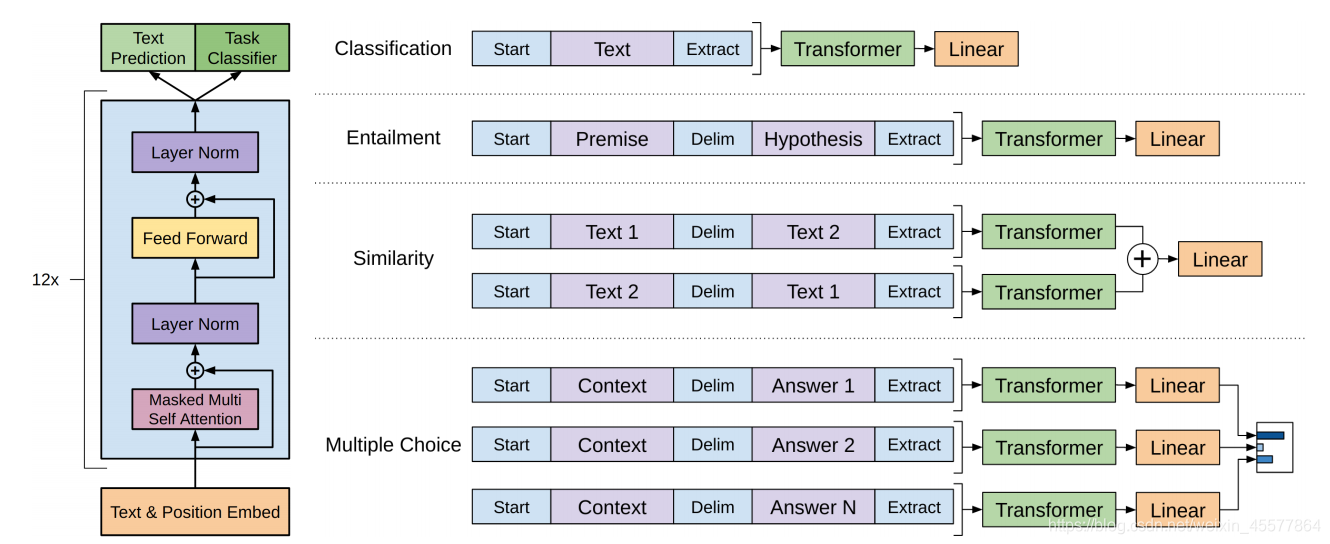
1. enter
2. Embedding
3. Multi-layer transformer block (12 layers)
4. Get two output results
5. calculate loss
6. backpropagation
7. update parameters

2.The following mainly introduces the block layer of Embedding and 3.transformer in the above steps

Embedding

The Embedding layer is a fully connected layer that takes one hot as input and the middle layer nodes as word vector dimensions. And the parameter of this fully connected layer is a "word vector table". Realize the transformation of text input dimension.

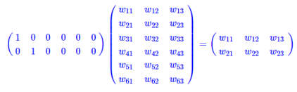
Embedding operation (here refers to text embedding) is actually a table lookup operation. One hot matrix multiplication is like a table lookup, so it directly uses the table lookup as an operation instead of writing it into a matrix for calculation. The amount of calculation is greatly reduced. It is emphasized again that the reduction in the amount of computation is not due to the emergence of word vectors, but because the one hot matrix operation is simplified to a table lookup operation.

code part

 def input_emb(self,seqs, segs):
        # device = next(self.parameters()).device
        # self.position_emb = self.position_emb.to(device)
        return self.word_emb(seqs) + self.segment_emb(segs) + self.position_emb

Including text embed and position embed

1. text embed

self.word_emb = nn.Embedding(n_vocab,model_dim)
self.word_emb.weight.data.normal_(0,0.1)

self.segment_emb = nn.Embedding(num_embeddings= max_seg, embedding_dim=model_dim)
self.segment_emb.weight.data.normal_(0,0.1)

The text embed part calls nn.Embedding to construct a word/segment vector matrix, and look up the table to achieve dimensionality reduction.

2. position embed

self.position_emb = torch.empty(1,max_len,model_dim)
nn.init.kaiming_normal_(self.position_emb,mode='fan_out', nonlinearity='relu')
self.position_emb = nn.Parameter(self.position_emb)

Position embed initializes a matrix containing the length of the input sequence as a dimension, and then uses it as a parameter to train and learn position information.

Transformer's block layer

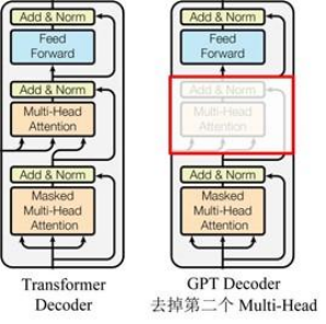
From the upper right figure, the block contained in GPT is similar to the Decoder of Transformer. Each block contains two sublayers:

1. Sublayer1: Masked Multi-Head Attention (mask multi-head attention layer)
2. Sublayer2: Feed Forward Network (FFN layer)

After each sublayer, there are residual connections and normalization operations

sublayer1: mask multi-head attention layer

输入: q, k, v, mask
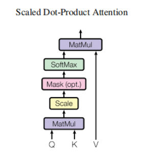
计算注意力(如下图左所示)：

1. Linear (matrix multiplication)
2. Scaled Dot-Product Attention
3. Concat (the result of multiple attentions)
4. Linear (matrix multiplication)

残差连接和归一化操作：Dropout operation → residual connection → layer normalization operation

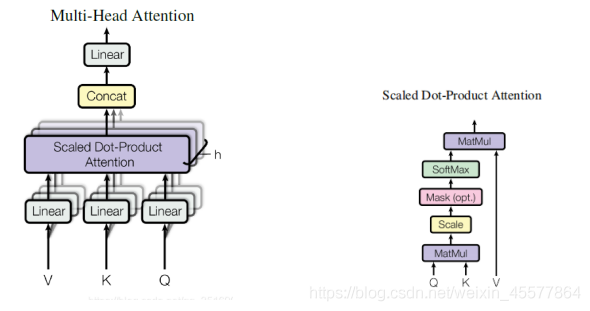
The left image in the above figure introduces the calculation process of the entire attention layer

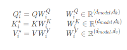
1. matrix multiplication

Multiply the input Q, K, V with the matrix to get new Q, K, V

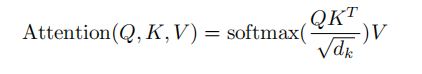
2. Scaled Dot-Product Attention

The name of this operation looks very long, but it is actually the process of dot multiplication + zoom + mask (optional) + Softmax + dot multiplication to calculate the attention value. The first step: dot multiplication of the
transposition of Q and K, and calculate Q and K Similarity
Step 2: Scaling, divided by a scale factor
Step 3: Part of the value in the Mask matrix (optional, this operation is available in GPT)
Step 4: Softmax, converted to the probability of each token
Step 5: The matrix value after Softmax is multiplied by the V value, and each value is weighted by probability to obtain the attention score.


Supplement:
Mask operation: masked_fill_(mask, value)
mask operation, fills the element in the tensor corresponding to the value 1 in the mask with value. The shape of the mask must match the shape of the tensor to be filled. (Here, -inf padding is used, so that the softmax becomes 0, which is equivalent to not seeing the following words)
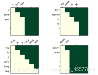
The mask operation in the transformer

Visualization matrix after mask:
The intuitive understanding is that each word can only see the word before it (because the purpose is to predict the future word, if you see it, you don’t need to predict it)

3. Concat operation

Combining the results of multiple attention heads is actually to transform the matrix: permute, reshape operations, and dimensionality reduction depending on the specific situation. (As shown in the red box in the figure below)

context = torch.matmul(self.attention,v)    # [n, num_head, step, head_dim]
context = context.permute(0,2,1,3)          # [n, step, num_head, head_dim]
context = context.reshape((context.shape[0], context.shape[1],-1))  
return context  # [n, step, model_dim]

4. matrix multiplication

A Linear layer that linearly transforms the attention results

Code for the entire mask multi-head attention layer

def forward(self,q,k,v,mask,training):
        # residual connect
        residual = q
        dim_per_head= self.head_dim
        num_heads = self.n_head
        batch_size = q.size(0)

        # 1.线性变换，linear projection
        key = self.wk(k)    # [n, step, num_heads * head_dim]
        value = self.wv(v)  # [n, step, num_heads * head_dim]
        query = self.wq(q)  # [n, step, num_heads * head_dim]

        # split by head
        query = self.split_heads(query)       # [n, n_head, q_step, h_dim]
        key = self.split_heads(key)
        value = self.split_heads(value)  # [n, h, step, h_dim]
        
        #2.3 Scaled Dot-Product Attention计算注意力分数 + Concat连接多头注意力
        context = self.scaled_dot_product_attention(query,key, value, mask)    # [n, q_step, h*dv]
        
        #4.Linear层，对注意力结果线性变换
        o = self.o_dense(context)   # [n, step, dim]
        
        #残差连接和归一化操作
        o = self.o_drop(o)
        o = self.layer_norm(residual+o)
        return o

Note that the residual connection and normalization operations are performed at the end, including:

1. Dropout operation
2. residual connection
3. layer normalization operation

sublayer2: FFN feedforward network

Mainly a multi-layer perceptron structure

1. Linear layer (matrix multiplication)
2. relu function activation
3. Linear layer (matrix multiplication)

Afterwards, the residual connection and normalization operations were also performed, including:

1. Dropout operation
2. residual connection
3. layer normalization operation

class PositionWiseFFN(nn.Module):
    def __init__(self,model_dim, dropout = 0.0):
        super().__init__()
        dff = model_dim*4
        self.l = nn.Linear(model_dim,dff)
        self.o = nn.Linear(dff,model_dim)
        self.dropout = nn.Dropout(dropout)
        self.layer_norm = nn.LayerNorm(model_dim)

    def forward(self,x):
        #1.2.线性层 + relu
        o = relu(self.l(x))
        #3.线性层
        o = self.o(o)
        #4.dropout
        o = self.dropout(o)
		#5.6.残差连接 + 层归一化
        o = self.layer_norm(x + o)
        return o    # [n, step, dim]